Graph Convolutional Networks
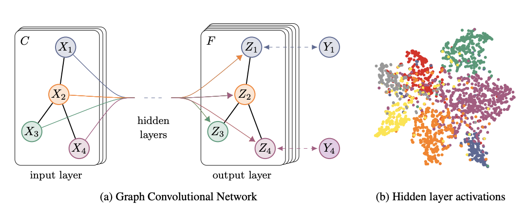
In the previous blogs we’ve looked at graph embedding methods that tried to capture the neighbourhood information from graphs. While these methods were quite successful in representing the nodes, they could not incorporate node features into these embeddings. For some tasks this information might be crucial, so today we’ll cover Graph Convolutional Networks (GCN) which can use both - graph and node feature information. As you could guess from the name, GCN is a neural network architecture that works with graph data. The main goal of GCN is to distill graph and node attribute information into the vector node representation aka embeddings. Below you can see the intuitive depiction of GCN from Kipf and Welling (2016) paper.
For this blog, I’ll be heavily using stellargraph library (docs) and their implementation of GCN. They provide excellent working notebooks here, so if you’re just interested in applying these methods, feel free to read their own notebooks instead. For this article, my goal is to dive under the hood of GCNs and provide some intuition into what is happening in each layer. I will show you then how to apply this model to the real-world dataset. You can get the full notebook with code in my github repo
Data
Let’s start by reading in data. Similar to the previous blogs, I’ll be using github dataset from this repository, so make sure to download the data and star the repository. We’re going to classify github users into web or ML developers. In this dataset, nodes are github developers who have starred more than 10 repositories, edges represent mutual following, and features are based on location, starred repositories, employer, and email.
edges_path = 'datasets-master/git_web_ml/git_edges.csv'
targets_path = 'datasets-master/git_web_ml/git_target.csv'
features_path = 'datasets-master/git_web_ml/git_features.json'

# Read in edges
edges = pd.read_csv(edges_path)
edges.columns = ['source', 'target'] # renaming for StellarGraph compatibility

# Read in features
with open(features_path) as json_data:
    features = json.load(json_data)

max_feature = np.max([v for v_list in features.values() for v in v_list])
features_matrix = np.zeros(shape = (len(list(features.keys())), max_feature+1))

i = 0
for k, vs in tqdm(features.items()):
    for v in vs:
        features_matrix[i, v] = 1
    i+=1

node_features = pd.DataFrame(features_matrix, index = features.keys()) # into dataframe for StellarGraph

# Read in targets
targets = pd.read_csv(targets_path)
targets.index = targets.id.astype(str)
targets = targets.loc[features.keys(), :]
We’ve just read in the data about 37700 developers. There are 289003 edges between these developers and they are based on mutual followership. In addition, each developer (node) has 4005 features. About 75% of users are web developers and 25% are ML developers.
StellarGraph Data
stellargraph has its own graph data structure that has a lot of cool functionalities and is required to work with their API. Transforming your data into StellarGraph is really simple, you just provide the node features and edges dataframes to the StellarGraph function. This data type also supports weighted edges, heterogeneous node and edge types, and directed graphs.
G = sg.StellarGraph(node_features, edges.astype(str))
print(G.info())
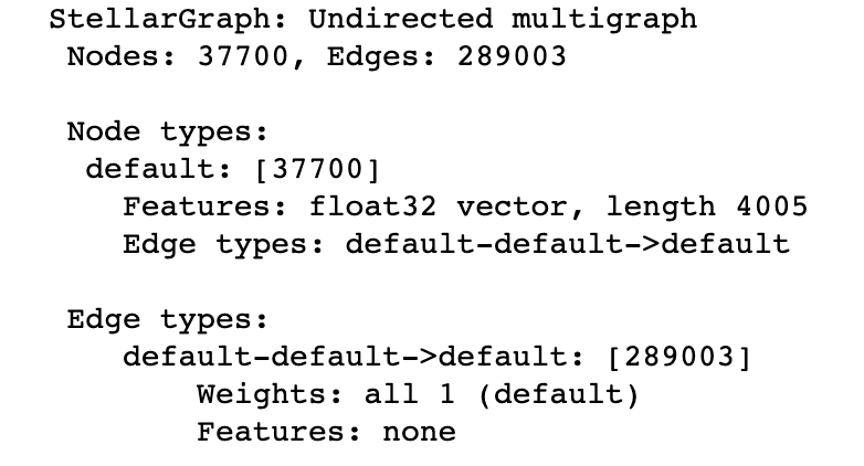
As you can see from the information printed, we’ve read in our data correctly. As with any other ML task, we need to split our data into the train/validation/test sets to make sure that we fairly evaluate our model. GCN is a semi-supervised model meaning that it needs significantly less labels than purely supervised models (e.g. Random Forest). So, let’s imaging the we have only 1% of data labeled which is about 400 developers. We’re going to use 200 developers for training, and 200 developers for validation in this scenario. Everything else will be used for testing.
train_pages, test_pages = train_test_split(targets, train_size=200)
val_pages, test_pages = train_test_split(test_pages, train_size=200)
print(train_pages.shape, val_pages.shape, test_pages.shape)

# Should print: ((200, 3), (200, 3), (37300, 3))
Data Pre-processing
First, let’s pre-process our labels data. Since we’re working with neural networks we need to one-hot-encode the labels. In the binary classification problem (like ours) we don’t actually have to do this, since we can just use sigmoid activation function at the final layer. But I’ll still show you how you’d do it for the multi-class classification problem.
target_encoding = LabelBinarizer()

train_targets = target_encoding.fit_transform(train_pages['ml_target'])
val_targets = target_encoding.transform(val_pages['ml_target'])
test_targets = target_encoding.transform(test_pages['ml_target'])
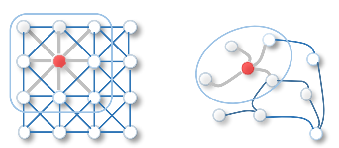
Pre-processing of the feature and graph data is a bit more complicated. This part is key for GCNs to work. To understand what kind of pre-processing we need to do, let’s take a look at what the Graph Convolutional Layer will be doing. What we want is to somehow aggregate the feature information from the neighbouring nodes because we want to learn the embeddings that reflect graph neighbourhoods. In Convolutional Neural Networks, which are usually used for image data, this is achieved using convolution operations with pixels and kernels. The pixel intensity of neighbouring nodes (e.g. 3x3) gets passed through the kernel that averages the pixels into a single value. It works well with image data because the neighbours are ordered and fixed in size. We don’t have these qualities with graphs so we need to come up with an alternative. You can see this difference illustrated below using the visualisation from Wu et al. (2019) survey on Graph Neural Networks.
The alternative is to use the idea of information passing by multiplying the hidden state by the adjacency matrix. If you recall from this post about label propagation, adjacency matrix denotes connections between the nodes. Hence, by multiplying the hidden state (or node features in the first layer) by it, we are sort of applying a mask and aggregating only the information from neighbouring nodes. Zak Jost has made a great video explaining these concepts in detail, so if you’re a bit unclear about why we need to multiply by the adjacency matrix, make sure to check out his video.
More formally, the Graph Convolutional Layer can be expressed using this equation: \[ H^{(l+1)} = \sigma(\tilde{D}^{-1/2}\tilde{A}\tilde{D}^{-1/2}{H^{(l)}}{W^{(l)}}) \]
In this equation:
- \(H\) - hidden state (or node attributes when \(l\) = 0)
- \(\tilde{D}\) - degree matrix
- \(\tilde{A}\) - adjacency matrix (with self-loops)
- \(W\) - trainable weights
- \(\sigma\) - activation function
- \({l}\) - layer number
As you can see, there are 2 parts of this equation - non-trainable (with D, A) and trainable (with H, A). The non-trainable part is called the normalised adjacency matrix and we’ll see how to calculate it below. You might have noticed that if we remove the non-trainable part, we’re left with simple dense layer. By multiplying hidden state with the normalised adjacency matrix, we are aggregating the neighbouring features as discussed above. The final question to answer is - why do we need to normalise the adjacency matrix? The intuitive explanation is that we want to discount the “contribution” of node features (or hidden states) from the highly connected nodes, as they are not that important. More formally, putting the adjacency matrix between two \(\tilde{D}^{1/2}\) results in scaling each adjacency value by \(\frac{1}{\sqrt{D_iD_j}}\) where \(i\) and \(j\) are some connected nodes. Hence, when the connected nodes have a lot of other connections (i.e. \(D\) is large), features get multiplied by a smaller value and are discounted.
Our task now is to pre-compute the non-trainable part, so let’s see how to do it. stellargraph implements these computations in sparse format because of speed, so we’ll follow their step and use their implementation.
# Get the adjacency matrix
A = G.to_adjacency_matrix(weighted=False)

# Add self-connections
A_t = A + sp.diags(np.ones(A.shape[0]) - A.diagonal())

# Degree matrix to the power of -1/2
D_t = sp.diags(np.power(np.array(A.sum(1)), -0.5).flatten(), 0)

# Normalise the Adjacency matrix
A_norm = A.dot(D_t).transpose().dot(D_t).todense()
Great, now you know how to pre-process the data for your GCN. There’s a couple more formalities we need to take care of before modelling:
- Get the new indices of train, val and test sets - required by model to calculate loss
- Add a dimension to our data - required by Keras to properly work
# Define the function to get these indices
def get_node_indices(G, ids):
    # find the indices of the nodes
    node_ids = np.asarray(ids)
    flat_node_ids = node_ids.reshape(-1)

    flat_node_indices = G.node_ids_to_ilocs(flat_node_ids) # in-built function makes it really easy
    # back to the original shape
    node_indices = flat_node_indices.reshape(1, len(node_ids)) # add 1 extra dimension

    return node_indices

# Get indices
train_indices = get_node_indices(G, train_pages.index)
val_indices = get_node_indices(G, val_pages.index)
test_indices = get_node_indices(G, test_pages.index)

# Expand dimensions
features_input = np.expand_dims(features_matrix, 0)
A_input = np.expand_dims(A_norm, 0)

y_train = np.expand_dims(train_targets, 0)
y_val = np.expand_dims(val_targets, 0)
y_test = np.expand_dims(test_targets, 0)
Now that data is normalised and in the right shape, we can move to modelling.
GCN Model
As you can see in the equation above, the GCN layer is nothing more but the multiplication of inputs, weights, and the normalised adjacency matrix. You can see this in the implementation of stellargraph’s GraphConvolution layer on github in lines 208 and 209. Since we know now what happens under the hood, let’s simply import the layer and use it in our architecture.
from stellargraph.layer.gcn import GraphConvolution, GatherIndices

# Initialise GCN parameters
kernel_initializer="glorot_uniform"
bias = True
bias_initializer="zeros"
n_layers = 2
layer_sizes = [32, 32]
dropout = 0.5
n_features = features_input.shape[2]
n_nodes = features_input.shape[1]
First of all, let’s initialise the Input layers with the correct shapes to receive our 3 inputs:
- Features matrix
- Train/Val/Test indices
- Normalised adjacency matrix
# Initialise input layers
x_features = Input(batch_shape=(1, n_nodes, n_features))
x_indices = Input(batch_shape=(1, None), dtype="int32")
x_adjacency = Input(batch_shape=(1, n_nodes, n_nodes))
x_inp = [x_features, x_indices, x_adjacency]
Now, we can build a model with 2 GCN dropout layers. Each layer will have 32 nodes which should be enough to transform the data into useful embeddings.
# Build the model
x = Dropout(0.5)(x_features)
x = GraphConvolution(32, activation='relu',
                     use_bias=True,
                     kernel_initializer=kernel_initializer,
                     bias_initializer=bias_initializer)([x, x_adjacency])
x = Dropout(0.5)(x)
x = GraphConvolution(32, activation='relu',
                     use_bias=True,
                     kernel_initializer=kernel_initializer,
                     bias_initializer=bias_initializer)([x, x_adjacency])

x = GatherIndices(batch_dims=1)([x, x_indices])
output = Dense(1, activation='sigmoid')(x)

model = Model(inputs=[x_features, x_indices, x_adjacency], outputs=output)

# Print out the summary
model.summary()
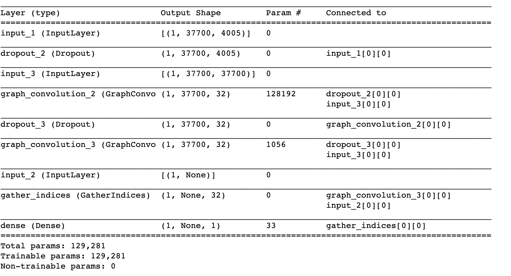
With the model defined, we can now compile it and train as usual Keras model. If you’re not familiar with the Keras interface, I recommend checking their tutorials here.
# Compile the model
model.compile(
    optimizer=optimizers.Adam(lr=0.01),
    loss=losses.binary_crossentropy,
    metrics=["acc"],
)

# Early stopping callback
es_callback = EarlyStopping(monitor="val_loss", patience=10, restore_best_weights=True)

# Fit the model
history = model.fit(
    x = [features_input, train_indices, A_input], # 3 inputs - features matrix, train indices, normalised adjacency matrix
    y = y_train,
    batch_size = 32,
    epochs=200,
    validation_data=([features_input, val_indices, A_input], y_val),
    verbose=1,
    shuffle=False,
    callbacks=[es_callback],
)
It will take some time to train the model as this implementation is not very optimised. If you use the stellargraph API fully (example below) the training process will be a lot faster.
Model Evaluation
Now that we have the trained model, let’s evaluate its accuracy on the test set we’ve set aside.
# Function to evaluate
def evaluate_preds(true, pred):
auc = roc_auc_score(true, pred)
pr = average_precision_score(true, pred)
bin_pred = [1 if p > 0.5 else 0 for p in pred]
f_score = f1_score(true, bin_pred)
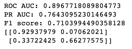
print('ROC AUC:', auc)
print('PR AUC:', pr)
print('F1 score:', f_score)
print(confusion_matrix(true, bin_pred, normalize='true'))
return auc, pr, f_score
auc, pr, f_score = evaluate_preds(test_targets.ravel(),test_preds[0].ravel())

We’re getting a ROC AUC score of 0.89 with just 200 labelled examples, not bad at all. Let’s visualise what the model has learned by accessing the embeddings before the classification layer.
# Define the embedding model
embedding_model = Model(inputs=x_inp, outputs=model.layers[-2].output)

# Get indices of all nodes
all_indices = get_node_indices(G, targets.index)

#Get embeddings
emb = embedding_model.predict([features_input, all_indices, A_input])
print(emb.shape)
# Shape: (1, 37700, 32)

# UMAP for visualisation
u = umap.UMAP(random_state=42)
umap_embs = u.fit_transform(emb[0])

#Plot the embeddingsembe
plt.figure(figsize=(20,10))
ax = sns.scatterplot(x = umap_embs[:, 0], y = umap_embs[:, 1], hue = targets['ml_target'])
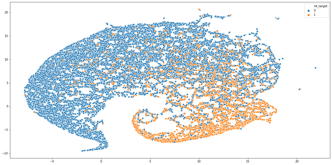
As you can see, two classes are quite distinctly clustered in the opposite sides of the graph. Yet, there’s some degree of mixing in the centre of the plot, which can be expected because ML and web developers still have a lot in common.
Adding More Data
To make these experiments faster and less complicated, let’s now use the StellarGraph API fully. Since you understand what’s happening under the hood, there’s nothing wrong with making your life easier! We’re going to run the experiment with 1000 labelled nodes but feel free to choose your own parameters here.
# 1000 training examples
train_pages, test_pages = train_test_split(targets, train_size=1000)
val_pages, test_pages = train_test_split(test_pages, train_size=500)

train_targets = target_encoding.fit_transform(train_pages['ml_target'])
val_targets = target_encoding.transform(val_pages['ml_target'])
test_targets = target_encoding.transform(test_pages['ml_target'])
Remember all the preprocessing we had to do above? Well, StellarGraph actually takes care of this for you. All you need to do is to initialise and use the BatchGenerator object.
# Initialise the generator
generator = FullBatchNodeGenerator(G, method="gcn")

# Use the .flow method to prepare it for use with GCN
train_gen = generator.flow(train_pages.index, train_targets)
val_gen = generator.flow(val_pages.index, val_targets)
test_gen = generator.flow(test_pages.index, test_targets)

# Build necessary layers
gcn = GCN(
    layer_sizes=[32, 32], activations=["relu", "relu"], generator=generator, dropout=0.5
)

# Access the input and output tensors
x_inp, x_out = gcn.in_out_tensors()

# Pass the output tensor through the dense layer with sigmoid
predictions = layers.Dense(units=train_targets.shape[1], activation="sigmoid")(x_out)

model = Model(inputs=x_inp, outputs=predictions)
model.compile(
    optimizer=optimizers.Adam(lr=0.01),
    loss=losses.binary_crossentropy,
    metrics=["acc"],
)
You can see that the stellargraph integrates with Keras very seamlessly which makes working with it so straightforward. Now, we can train the model in the same way we did before. The only difference is that we don’t need to worry about providing all the inputs to the model, as the generator objects take care of it.
# Train the model
history = model.fit(
    train_gen,
    epochs=200,
    validation_data=val_gen,
    verbose=2,
    shuffle=False,  # this should be False, since shuffling data means shuffling the whole graph
    callbacks=[es_callback],
)

new_preds = model.predict(test_gen)

auc, pr, f_score = evaluate_preds(test_targets.ravel(),new_preds[0].ravel())
The test scores have imporved as expected, so adding more data can still lead to a better model.
Conclusion
GCNs are a powerful deep neural network architecture that allows you to combine the feature and graph neighbourhood information. This is achieved by multiplying previous layer values by the normalised adjacency matrix which acts as a convolutional filter. As a result of this multiplication, the features of neighbouring nodes get aggregated and useful embeddings can be learned using back-propagation as usual.
I hope that by now you know not only how to apply GCNs to your data but also feel more confident about what’s happening under the hood. Thank you for reading, and if you have any questions or comments, feel free to reach out using my email or LinkedIn.
![]()