Finding Mature Language in Twitch with Label Propagation

Tell me who your friends are

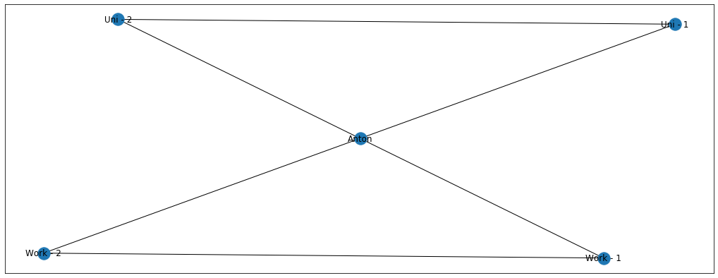
There’s this famous saying - “Tell me who your friends are, and I will tell you who you are”. Not sure how generalisable this statement is but it is useful in explaining label propagation. Let’s say that I have 4 friends - 2 from university and 2 from work.

Imagine now that my friends from university and from work are giant football fans and talk about it all the time. I, on the other hand, am still undecided whether I like the game or not. Let’s denote football = blue and undecided = grey

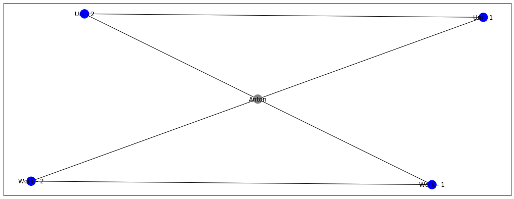
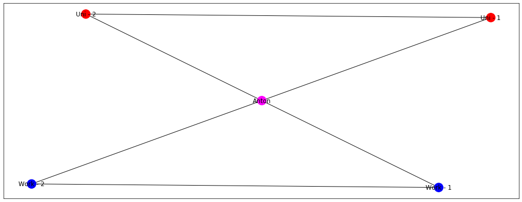
Just by looking at this graph, it becomes logical that node Anton should also be coloured blue! This is exactly the idea of label propagation - if everyone in my surrounding likes football, I’m very likely to like it as well. Which makes intuitive sense, right? My colleagues and friends are going to discuss it all the time, watch games togethers, and play it themselves. At some point, I’m likely to give in and just join a game or two, until I become a massive fan myself. But let’s say, that my colleagues from work still like football, but my friends from university now started to enjoy boxing more. Let’s denote boxing = red.

Now it’s more challenging, right? Will my node become blue or red? Well, probably something in the middle because I want to be a part of the both of the groups. Label propagation algorithms ensure that the labels of your surrounding are sort of averaged and the node Anton gets something of a magenta colour.

Now that we have an intuitive understanding of label propagation, let’s start working with a larger graph.

Generating Graph Data

Before working with large real world datasets, I want to show you the power of label propagation on the limited fake dataset. The real-life graphs are usually huge with thousands of nodes and hundreds of thousands of edges, so it’ll be easier to digest the algorithm using this limited example.

import networkx as nx

G = nx.gnp_random_graph(100, 0.02, seed=42) # Graph size = 100, probability that 2 nodes are connected - 2%
pos = nx.spring_layout(G, seed=42) # To be able to recreate the graph layout
nx.draw_networkx(G, pos=pos) # Plot the graph

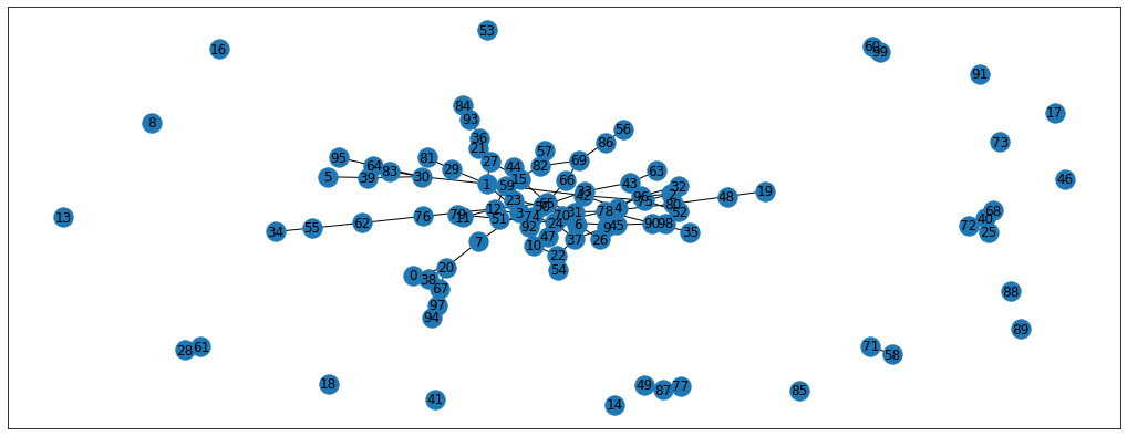
Cool, we now have 1 large graph and some nodes that are not connected. Let’s delete these unconnected nodes, as there’s no way to propagate the information to them (at least without any additional data)

subgraph_nodes = list(nx.dfs_preorder_nodes(G, 7)) #Gets all the nodes in the graph that node 7 belongs to. 
G = G.subgraph(subgraph_nodes)
pos = nx.spring_layout(G, seed=42)
nx.draw_networkx(G, pos=pos, cmap='coolwarm')

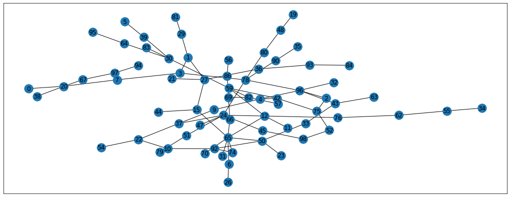
Much better! This graph is absolutely random, so there’s no labels associated with it. Manually, I’m going to pick 10 nodes, and I will label them as 1 if they come from the right side of the graph and -1 if from the left side. This way, we’re going to have some of the nodes labelled and we’ll see the label propagation in action.

known_nodes = np.array([76, 96, 80, 93, 45, 37, 10, 1, 7, 30]) #picked more or less randomly
unknown_nodes = np.array([n for n in G.nodes if n not in known_nodes])

known_y = np.array([1, 1, 1, 1, 1, -1, -1, -1, -1, -1])
unknown_y = np.array([0 for i in range(len(unknown_nodes))])

init_labels = dict(zip(np.append(known_nodes, unknown_nodes), np.append(known_y,unknown_y)))
init_colors = [init_labels[i] for i in list(G.nodes)]
nx.draw_networkx(G, pos=pos, node_color=init_colors, cmap='coolwarm')

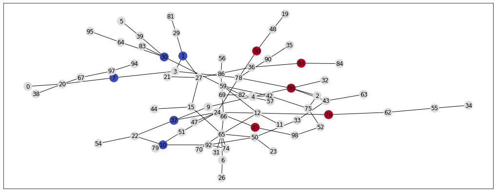
Given this set of label, nodes, and edges, our task is to assign some sort of label to the unlabelled nodes. In other words, given that we know what some of the people in the network like (e.g. football or boxing) and with whom they are friends, we need to guess whether their friends better prefer football or boxing. To answer this question, I’m going to explain this Label Propagation algorithm (Zhu 2002).

Graph Basics - Adjacency and Transition Matrices

To understand what this algorithm does, I need to introduce a new concepts - Adjacency Matrix. Adjacency matrix simply says to which nodes each node is connected. It’s a way to represent a graph using data structures that can be used in computations. We can get an adjacency matrix for our graph using networkx functions.

A = np.array(nx.adj_matrix(G).todense())
A_df = pd.DataFrame(A, index=G.nodes(), columns=G.nodes())
A_df.head()

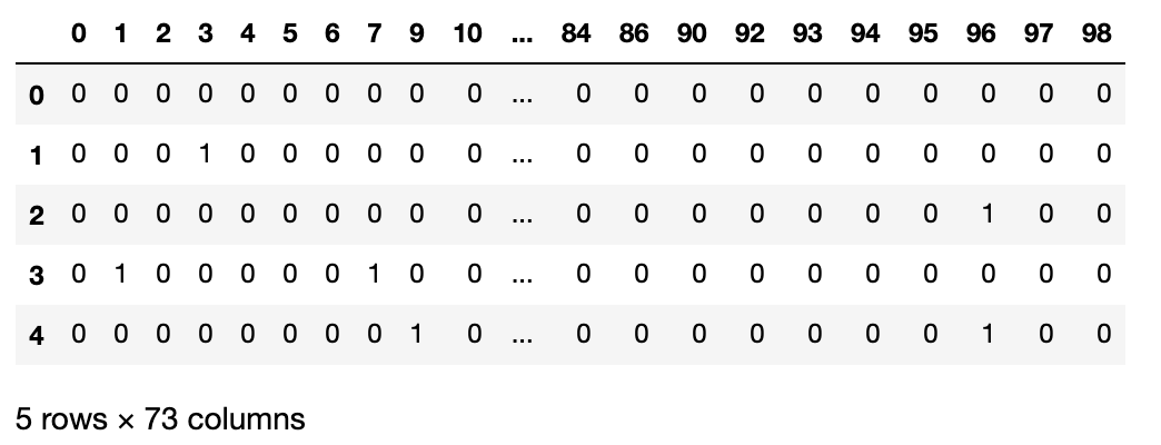
Using this matrix we can check which nodes are connected via the edges. For example, let’s see to which nodes the node 29 is connected. If you look at the graph, it should be connected to the nodes 81 and 1

A_df.loc[29, :][A_df.loc[29, :]  == 1]
#Expected output:
# 1     1
# 81    1
# Name: 29, dtype: int64

Having this matrix representation of the graph we can do so much more! For example, we can calculate the degree matrix i.e. to how many nodes each node is connected. Also, we can calculate the transition matrix which in our friends network analogy can mean - what’s the probability that a particular person is going to talk to another person in this network?

 T = np.matrix(A / A.sum(axis=1, keepdims=True))
T_df = pd.DataFrame(T, index=G.nodes(), columns=G.nodes())
T_df.loc[29, :][T_df.loc[29, :]  != 0]
#Expected output:
# 1    0.50000
# 81   0.50000
# Name: 29, dtype: float64

Here we can see that because node 29 was connected to nodes 1 and 81, they both get probability of 50%. We could alter this with some kind of connection weights to make some connections more probable than another. E.g. if I talked to my friends from work more frequently, I’d want the graph to represent this as well, to ensure that the labels get propagated accordingly. And that’s basocially all the prep for for this algorithm!

Label Propagation Algorithm

The actual algorithm can be described in these 6 steps:

1. Order your nodes in a way, that the nodes with known labels are first
2. Calculate the adjacency matrix
3. Calculate transition matrix
4. Make known nodes absorbing:
   • Set probability of going from known node to the same known node as 1
   • Set all the other probabilities as 0
   • This way, the probability of going from e.g. node 1 to node 1 is 100%
5. Update the labels by multiplying the known labels with the resulting transition matrix
6. Repeat until the labels stop changing

Don’t feel overwhelmed with these steps (I know I was), instead examine the code implementation and feel free to read the paper for better intuition on why it works.

def label_propagation(G, Y_init, known_nodes, unknown_nodes, threshold=0.01):
    # Step 1: order nodes
    ordered_nodes = list(known_nodes) + list(unknown_nodes) 
    
    # Step 2: adjacency matrix
    A = nx.adj_matrix(G, nodelist=ordered_nodes) 
    A = A.todense()
    A = np.array(A, dtype = np.float64)
    
    # Step 3: transition matrix
    T = A / A.sum(axis=1, keepdims=True)
    
    # Step 4: absorbing nodes
    T[:len(known_nodes), :] = 0
    T[:len(known_nodes), :len(known_nodes)] = np.identity(len(known_nodes)) 
    
    #Step 5 & 6: update labels until convergence
    labels = [Y_init] #stores the label progression for the animation
    Y1 = Y_init 
    for i in tqdm(range(1000)):
        Y0 = Y1
        Y1 = np.dot(T, Y0) #The actual probability update is happening here. 
        diff = np.abs(Y0 - Y1).sum() #calculate the difference between Y(t-1) and Y(t)
        Y1[:len(known_nodes)] = Y_init[:len(known_nodes)] #set the known labels back to their initial values
        labels.append(Y1)
        if i % 10 == 0:
            print('Total difference:', diff)
        if diff < threshold: #stopping criterion
            break
    
    return labels

With the algorithm defined, let’s run it and see the results.

Y_init = np.append(known_y, unknown_y) #remember, the known labels (nodes) should always go first
labels = label_propagation(G, Y_init, known_nodes, unknown_nodes, threshold=0.01) #run the algorithm
propagated_labels = dict(zip(np.append(known_nodes, unknown_nodes), labels[-1])) #create a dictionary node:label
propagated_colors = [propagated_labels[i] for i in list(G.nodes)] #color intensity for visualisation
nx.draw_networkx(G, pos=pos, node_color=propagated_colors,  cmap='coolwarm')

Here’s the animation of how the labels change with each iteration. Notice that the right hand side becomes noticeably more red which indicates that they have larger propagated labels. This is exactly what we’d expect from this algorithm, so we can say that it was successful in its task. Now that we understand label propagation and know how to apply it, let’s try it on Twitch dataset.

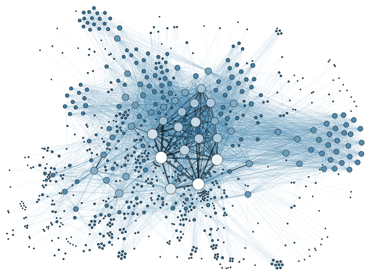
Twitch Dataset

To get this dataset you need to pull this github repository done by Benedek Rozemberczki (don’t forget to star it and check out his other cool graph repos). Find the datasets/twitch/ENGB/ folder, we’ll use all the files in there. It has 3 files:

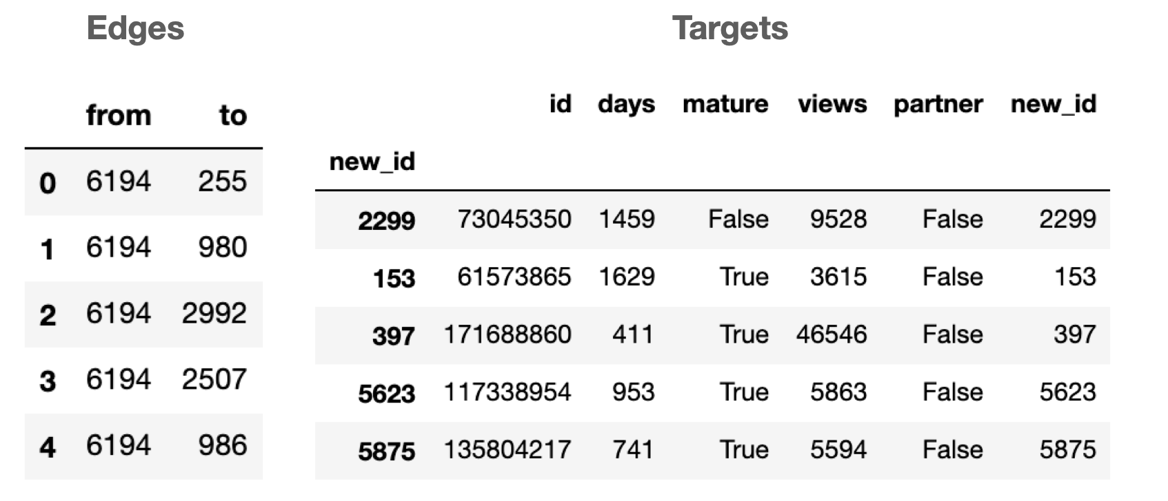
• edges.csv - 2 columns table that describes from which twitch user (node) to which user there’s a connection
• features.json - json file that stores different one-hot-encoded features of every twitch user in a graph
• targets.csv - a table that contains our binary target (“mature language”) for each twitch user

The csv files can be reain in simply using pandas.

import pandas as pd

edges_path = 'datasets-master/twitch/ENGB/ENGB_edges.csv'
targets_path = 'datasets-master/twitch/ENGB/ENGB_target.csv'

edges = pd.read_csv(edges_path)
display(edges.head())

targets = pd.read_csv(targets_path)
targets.index = targets.new_id
display(targets.head())

The json file is trickier to read in as the data is stored in the sparse binary format (i.e. it stores the column indices where the value is 1). Here’s the code to read it in:

import json
import numpy as np

# Reading the json as a dict
with open(features_path) as json_data:
    features = json.load(json_data)

#number of columns in features matrix
max_feature = np.max([v for v_list in features.values() for v in v_list])

#create empty array 
features_matrix = np.zeros(shape = (len(list(features.keys())), max_feature+1))
print(features_matrix.shape)
#Expected: (7126, 3170)

i = 0
for k, vs in features.items():
    for v in vs:
        features_matrix[i, v] = 1
    i+=1

#Get the targets in correct order
y = targets.loc[[int(i) for i in list(features.keys())], 'mature']

We’ve read in the data, so now we can build the graph from edges dataframe and propagate the labels.

#read in the graph
graph = nx.convert_matrix.from_pandas_edgelist(edges, "from", "to")

To be able to evaluate the accuracy of label propagation, let’s set aside some nodes as testset. In other words, we’ll do a train/test split just like we do with regular classification models. In addition, we’ll repeat the experiment 100 times to get more unbiased result of AUC score

aucs = []
for i in range(100):
    known = y.sample(n=int(0.8 * len(y))) # indices of known nodes
    known_nodes = known.index.values # and their values

    unknown = y[~y.index.isin(known.index)] # indices of unknown nodes
    unknown_nodes = unknown.index.values # and their values

    Y_init = [1 if y == True else 0 for y in known] + [0 for y in unknown] # ordered labels
    labels = label_propagation(graph, Y_init, known_nodes, unknown_nodes) # results of label propagation
    
    aucs.append(roc_auc_score(unknown.values, labels[-1][len(known_nodes):])) #auc score

print(np.mean(aucs))
print(np.std(aucs))

I got the average AUC of 0.578 and the standard deviation of 0.013. It’s definitely better than random (hurray!) but is it good? Since we have a meaningful features matrix we can actually built a simple supervised model and compare the performance of label propagation with this model. With the same split (80/20) I’ll build a Random Forest model and see what AUC score can we achieve.

rf_aucs = []
for i in tqdm(range(100)):
    X_train, X_test, y_train, y_test = train_test_split(features_matrix, y, test_size = 0.2)
    rf = RandomForestClassifier(n_estimators=50)
    rf.fit(X_train, y_train)
    y_preds = rf.predict_proba(X_test)
    rf_aucs.append(roc_auc_score(y_test, y_preds[:, 1]))

print(np.mean(rf_aucs))
print(np.std(rf_aucs))

For the Random Forest model I got the average AUC of 0.616 and the standard deviation of 0.014. The results of the supervised model are better but only marginally. This is really impressive as the Random Forest used thousands of features whereas the label propagation used only the information about node connections. One of the key advantages of graph algorithms is that they tend to need less labels, so weakly supervised learning is possible. The main disadvantage with label propagation is that we have to make an assumption that connected nodes are similar in attributes that we care about. This assumption usually holds, but we need to be aware of it.

Conclusion

I hope by now you understand the basics of working with graph data and know how to apply simple (yet effective) algorithm of label propagation. We saw it in action that only by using graph information we can achieve results close to the supervised model. This blog also gave a good basis for the more advance graph ML techniques that I’ll cover in my future blogs.