In the previous blog you saw how Graph Convolution Networks work and how you can apply them using stellargraph and Keras. It worked great, had quite a high accuracy score, and the embeddings made sense, so what else would we want? Well, one of the main disadvantages of GCNs is that they are not efficient for dynamic graphs. Every time a new node gets added, you’ll need to retrain the model and update the embeddings accordingly. This type of learning is called transductive and with large graphs it is not really feasible. So, in this blog I’ll cover GraphSAGE - an inductive deep learning model for graphs that can handle the addition of new nodes without retraining.
Data
For the ease of comparison, I’ll use the same dataset as in the last blog. You can download the data from this github repo and don’t forget to start it.
edges_path = 'datasets-master/git_web_ml/git_edges.csv'
targets_path = 'datasets-master/git_web_ml/git_target.csv'
features_path = 'datasets-master/git_web_ml/git_features.json'

# Read in edges
edges = pd.read_csv(edges_path)
edges.columns = ['source', 'target'] # renaming for StellarGraph compatibility

with open(features_path) as json_data:
    features = json.load(json_data)

max_feature = np.max([v for v_list in features.values() for v in v_list])
features_matrix = np.zeros(shape = (len(list(features.keys())), max_feature+1))

i = 0
for k, vs in tqdm(features.items()):
    for v in vs:
        features_matrix[i, v] = 1
    i+=1

node_features = pd.DataFrame(features_matrix, index = features.keys())

# Read in targets
targets = pd.read_csv(targets_path)
targets.index = targets.id.astype(str)
targets = targets.loc[features.keys(), :]

# Put the nodes, edges, and features into stellargraph structure
G = sg.StellarGraph(node_features, edges.astype(str))
Data Split
Since this model is inductive, to test it properly we’ll set aside 20% of the nodes and the model will never see them during the training process. In a way, we’ll just imaging that these 20% of github users have registered just after we’ve deployed our model.
labels_sampled = targets['ml_target'].sample(frac=0.8, replace=False, random_state=101)
G_sampled = G.subgraph(labels_sampled.index)

print('# nodes in full graph:', len(G.nodes()))
print('# nodes in sampled graph:', len(G_sampled.nodes()))
There should be 37700 nodes in the full graph and 30160 nodes after the holdout set was set aside.
Now, we can split the data into traditional train, validation, and test sets. Since GraphSAGE is a semi-supervised model, we can use a very small fraction of nodes for training.
# 5% train nodes
train_labels, test_labels = model_selection.train_test_split(
    labels_sampled,
    train_size=0.05,
    random_state=42,
)

# 20% of test for validation
val_labels, test_labels = model_selection.train_test_split(
    test_labels, train_size=0.2, random_state=42,
)
Now we have all we need to dive into GraphSAGE.
GraphSAGE
GraphSAGE was developed by Hamilton, Ying, and Leskovec (2017) and it builds on top of the GCNs (paper). The primary idea of GraphSAGE is to learn useful node embeddings using only a subsample of neighbouring node features, instead of the whole graph. In this way, we don’t learn hard-coded embeddings but instead learn the weights that transform and aggregate features into a target node’s embedding.
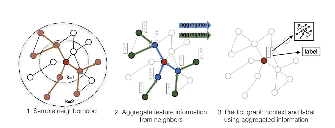
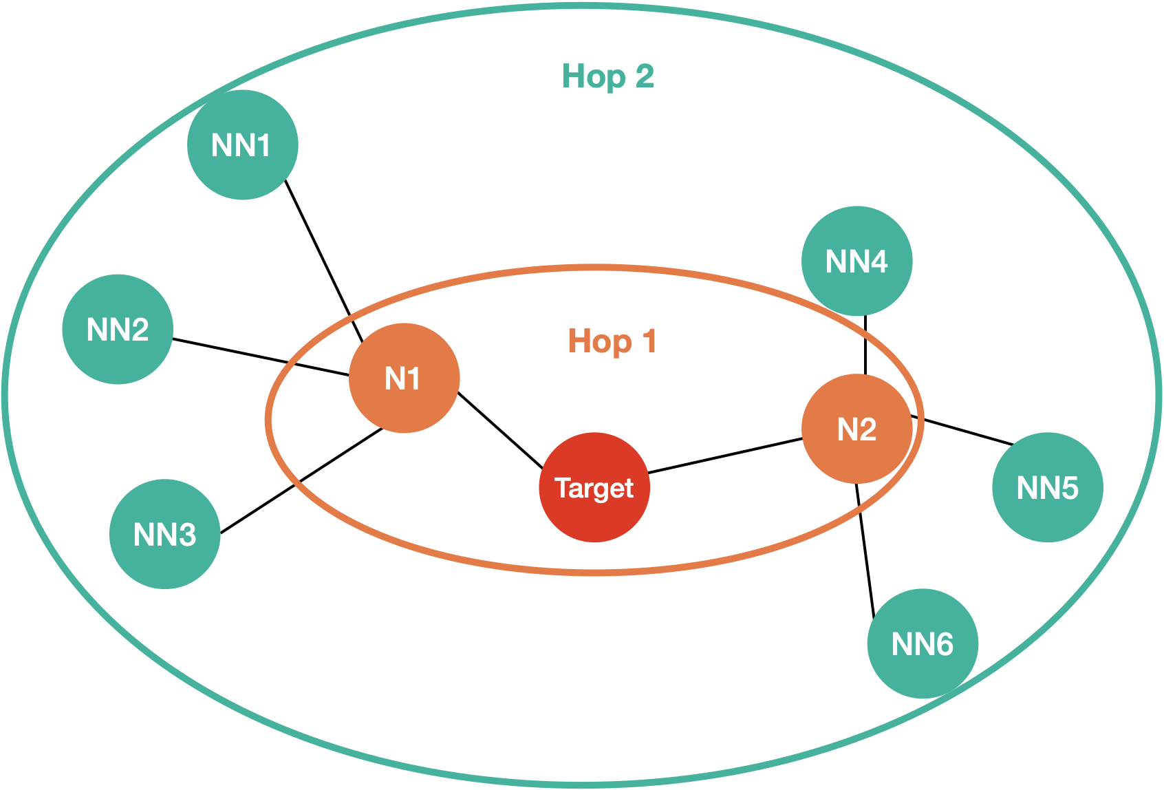
Sampling
Sampling is the first step in training GraphSAGE. Instead of using all the nodes as we did in GCN, we’re going to use only a subset of neighbouring nodes at different depth layers. The paper uses 25 neighbours in the first layer, and 10 neighbours in the second layer. Below you can see the sampling code for your intuition (hard-coded 2 layers) but in practice, I’m going to use the stellargraph sampler which is much faster and supports varying depths.
def depth_sampler(n, n_sizes):
    node_lists = []

    # First layer
    # get all neighbours
    neighbours = G_sampled.neighbor_arrays(n)
    # randomly choose neighbours
    if len(neighbours) > 0:
        neighbours_chosen = np.random.choice(neighbours, size=n_sizes[0])
    else:
        neighbours_chosen = np.full(n_sizes[0], -1)

    node_lists.append(list(neighbours_chosen))

    # Second Layer
    second_layer_list = []
    for node in neighbours_chosen:
        # get all neighbours
        if node != -1:
            neighbours = G_sampled.neighbor_arrays(node)
        else:
            neighbours = []
        # randomly choose neighbours
        if len(neighbours) > 0:
            neighbours_chosen = list(np.random.choice(neighbours, size=n_sizes[1]))
        else:
            neighbours_chosen = list(np.full(n_sizes[1], -1))

        second_layer_list += neighbours_chosen

    node_lists.append(second_layer_list)

    return node_lists
To visualise what this sampler is actually doing, let’s plot the sampled neighbourhood of a random node
np.random.seed(2)
# random node
rand_n = np.random.choice(G_sampled.nodes())
# sample 2 layers
sampled_nodes = depth_sampler(rand_n, [5, 5])
# plot
all_nodes = np.unique(sampled_nodes[0] + sampled_nodes[1] + [rand_n])
len(sampled_nodes[0]), len(sampled_nodes[1])

plt.figure(figsize=(20,10))
draw_networkx(G_sampled.subgraph(all_nodes).to_networkx(),
              node_color = ['#F1828D' if n == rand_n else '#FCD0BA' if n in set(sampled_nodes[0]) else '#8fb9A8' if n in set(sampled_nodes[1])  else 'grey' for n in all_nodes],
             node_size=2000,
             width=[2  if rand_n in e else 0.5 for e in G_sampled.subgraph(all_nodes).to_networkx().edges()],
             edge_color='grey')
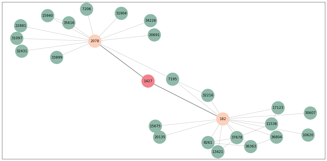
As you can see, our target node is 1427 (red). Its direct neighbours are nodes 2078 and 182 (orange) so only they get sampled. In turn, their neighbours (overall 23 green nodes) also get sampled and they all form the target node’s neighbourhood. This type of sampling is done for all the nodes and is used to construct inputs to the model. Note that some of these nodes were sampled multiple times. As I said above, we can actually use stellargraph generator object that does all of this for us.
# number of nodes per batch
batch_size = 50

# number of neighbours per layer
num_samples = [10, 10]

# generator
generator = GraphSAGENodeGenerator(G_sampled, batch_size, num_samples)

# Generators for all the data sets
train_gen = generator.flow(train_labels.index, train_labels, shuffle=True)
val_gen = generator.flow(val_labels.index, val_labels)
test_gen = generator.flow(test_labels.index, test_labels)
Aggregator
The aggregator takes neighbours of the previous layers and, you guessed it, aggregates it. In the paper they mention that it could be any kind of aggregating operation - simple averaging, pooling, or even LSTM. Here’s how the mean pooling works. Imagine you have the following graph:
Optional: Deep Dive
Note: The following section is going to be quite detailed, so if you’re interested in just applying the GraphSage feel free to skip the explanations and go to the StellarGraph Model section.
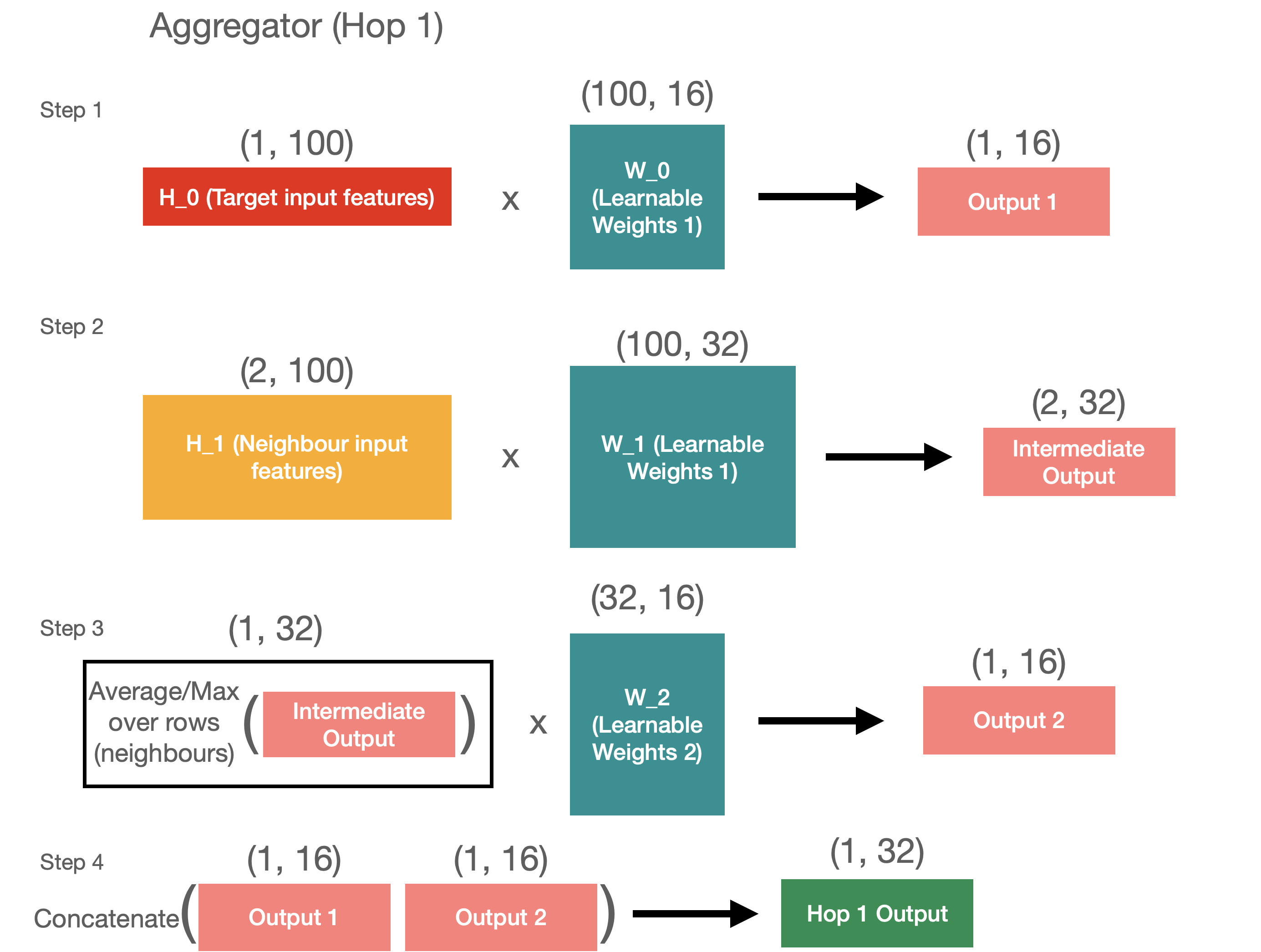
First, let’s start with the hop 1 aggregation. For hop 1 we have 2 inputs - target nodes and its neighbours.
# Initialise inputs
target = np.random.randn(1, 100) # example target input
H_1 = np.random.randn(2, 100) # example hop 1 neighbours
To aggregate these inputs, we want to translate each of them into 1 by 16 matrices and then concatenate them. It’s quite easy to do for the target node, as we just need to get the dot product of the target features with learnable matrix.
W_0 = np.random.randn(100, 16) # first learnable matrix

output_1 = np.dot(target, W_0)
print('Output 1 shape:', output_1.shape)
# Output 1 shape: (1, 16)
To aggregate the neighbour features, we have a few more steps. First, we need to distill the neighbours’ features into the target size of 32, and then we can average across the neighbours. We then have a new matrix with learnable weights that learns to translate the averaged values into the final output.
W_1 = np.random.randn(100, 32) # second learnable matrix
inter_output = np.dot(H_1, W_1)
print('Intermediate neighbour output shape:', inter_output.shape)
# Intermediate neighbour output shape: (2, 32)

averaged_inter_output = np.expand_dims(np.mean(inter_output, axis=0), axis=0) # average across neighbours
print('Averaged intermediate neighbour output shape:', averaged_inter_output.shape)
# Averaged intermediate neighbour output shape: (1, 32)

W_2 = np.random.randn(32, 16) # third learnable matrix
output_2 = np.dot(averaged_inter_output, W_2)
print('Output 2 shape:', output_2.shape)
# Output 2 shape: (1, 16)
Finally, we can concatenate 2 outputs into 1.
hop_1_output = np.concatenate([output_1, output_2], axis=1)
print('Hop 1 output shape:', hop_1_output.shape)
# Hop 1 output shape: (1, 32)
All of this is visualised in the diagram below for your reference.
Hop 1 aggregation is done. Now hop 2 follows the same approach but it takes the neighbours’ features and the neighbour neighbours’ features as inputs.
H_2 = np.random.randn(2, 3, 100) # example hop 2 neighbours

W_3 = np.random.randn(100, 16) # fourth learnable matrix
output_3 = np.dot(H_1, W_3)
print('Output 3 shape:', output_3.shape)
# Output 3 shape: (2, 16)

W_4 = np.random.randn(100, 32) # fifth learnable matrix
inter_output_2 = np.dot(H_2, W_4)
print('Intermediate neighbour output (hop 2) shape:', inter_output_2.shape)
# Intermediate neighbour output (hop 2) shape: (2, 3, 32)

averaged_inter_output_2 = np.mean(inter_output_2, axis=1) # average across neighbours
print('Averaged intermediate neighbour output (hop 2) shape:', averaged_inter_output_2.shape)
# Averaged intermediate neighbour output (hop 2) shape: (2, 32)

W_5 = np.random.randn(32, 16) # sixth learnable matrix
output_4 = np.dot(averaged_inter_output_2, W_5)
print('Output 2 shape:', output_4.shape)
# Output 2 shape: (2, 16)

hop_2_output = np.concatenate([output_3, output_4], axis=1)
print('Hop 2 output shape:', hop_2_output.shape)
# Hop 2 output shape: (2, 32)
Same as above, here’s the visual representation of what’s happening in the code block.

So now we have 2 outputs with shapes of (1, 32) and (2, 32). We can use these outputs as inputs to the second layer of aggregation. The operations we need to do are exactly the same as in the layer 1 but only for the first hop (as we only have 2 inputs).
W_6 = np.random.randn(32, 16) # seventh learnable matrix

l2_output_1 = np.dot(hop_1_output, W_6)
print('Layer 2 output 1 shape:', l2_output_1.shape)
# Layer 2 output 1 shape: (1, 16)

W_7 = np.random.randn(32, 32) # eight learnable matrix
l2_inter_output = np.dot(hop_2_output, W_7)
print('Layer 2 intermediate output shape:', l2_inter_output.shape)
# Layer 2 output 1 shape: (1, 16)

averaged_l2_inter_output = np.expand_dims(np.mean(l2_inter_output, axis=0), axis=0)
print('Averaged layer 2 intermediate neighbour output shape:', averaged_l2_inter_output.shape)
# Averaged layer 2 intermediate neighbour output shape: (1, 32)

W_8 = np.random.rand(32, 16) # ninth learnable matrix
l2_output_2 = np.dot(averaged_l2_inter_output, W_8)
print('Layer 2 output 2 shape:', l2_output_2.shape)
# Layer 2 output 2 shape: (1, 16)

l2_output = np.concatenate([l2_output_1, l2_output_2], axis=1)
print('Layer 2 (Final) output shape:', l2_output.shape)
# Layer 2 (Final) output shape: (1, 32)
And there we have it! All the neighbours and the target are aggregated into the embedding of size 32. Through the gradient descent, the network will find the optimal weights for the aggregation matrices (9 of them in this case) and we’ll have our inductive model.
Model
Now that you have an intution of how sampling and aggregation works, we can define network architecture using the following parameters.
layer_sizes = [32, 32] # embedding sizes at each layer
max_hops = 2 # number of hops (must be equal to len(layer_sizes))
feature_sizes = generator.graph.node_feature_sizes()
input_feature_size = feature_sizes.popitem()[1] # length of features vector
dims = [input_feature_size] + layer_sizes
neighbourhood_sizes = [1, 10, 100] # target, neighbours, neighbours' neighbours
aggregator = MeanPoolingAggregator # keras aggregation layer (explained above)
activations = ['relu', 'linear']
aggs = [aggregator(layer_sizes[l],
                  bias=True,
                  act=activations[l],
                  kernel_initializer="glorot_uniform",
                  )
       for l in range(max_hops)]
Take your time to go through the code below. There I’ve essentially unwrapped the GraphSAGE model class from stellargraph API to show you how the model gets built.
 # Create tensor inputs
x_inp = [Input(shape=(1, input_feature_size)), # target
         Input(shape=(10, input_feature_size)), # neighbours
         Input(shape=(100, input_feature_size))] # neighbours' neighbours

# Input becomes the first hidden layer
h_layer = x_inp

# ------------------------------------ Layer 1 ---------------------------------------
# Store the outputs here
layer_out = []

# --------------- Hop 1 ------------
# Layer takes the 10 neighbours of target node and Reshapes the tensor into (1, 10, 500) shape with dropout
neigh_in = Dropout(0.2)(
    Reshape((1, 10, input_feature_size)
)(h_layer[1])) # shape 1, 10, input_feature_size

# Aggregates the neighbours and target node itself into hidden layer with 32 neurons
layer_out.append(aggs[0]([Dropout(0.2)(h_layer[0]), neigh_in]))

# --------------- Hop 2 ------------
# Reshape the input of neighbours for the first layer (10 neighbours of 10 neighbours with 500 features)
neigh_in = Dropout(0.2)(
    Reshape((10, 10, input_feature_size)
)(h_layer[2]))

layer_out.append(aggs[0]([Dropout(0.2)(h_layer[1]), neigh_in]))

# Now the hidden state is the output of the previous layer
h_layer = layer_out

# ------------------------------------ Layer 2 ---------------------------------------
# Store the outputs here
layer_out = []

# --------------- Hop 1 ------------
# Layer takes the 10 neighbours of target node and Reshapes the tensor into (1, 10, 500) shape with dropout
neigh_in = Dropout(0.2)(
    Reshape((1, 10, 32)
)(h_layer[1])) # shape 1, 10, 32

layer_out.append(aggs[1]([Dropout(0.2)(h_layer[0]), neigh_in]))
# No hop 2 because we have aggregated everything we need

h_layer = layer_out
h_layer = Reshape((32,))(h_layer[0])

prediction = layers.Dense(units=1, activation="sigmoid")(h_layer)
model = Model(inputs = x_inp, outputs=prediction)

model.compile(
    optimizer=optimizers.Adam(lr=0.005),
    loss=losses.binary_crossentropy,
    metrics=[metrics.AUC(num_thresholds=200, curve='ROC'), 'acc'],
)

model.summary()
Here’s what you should see in the model summary report.
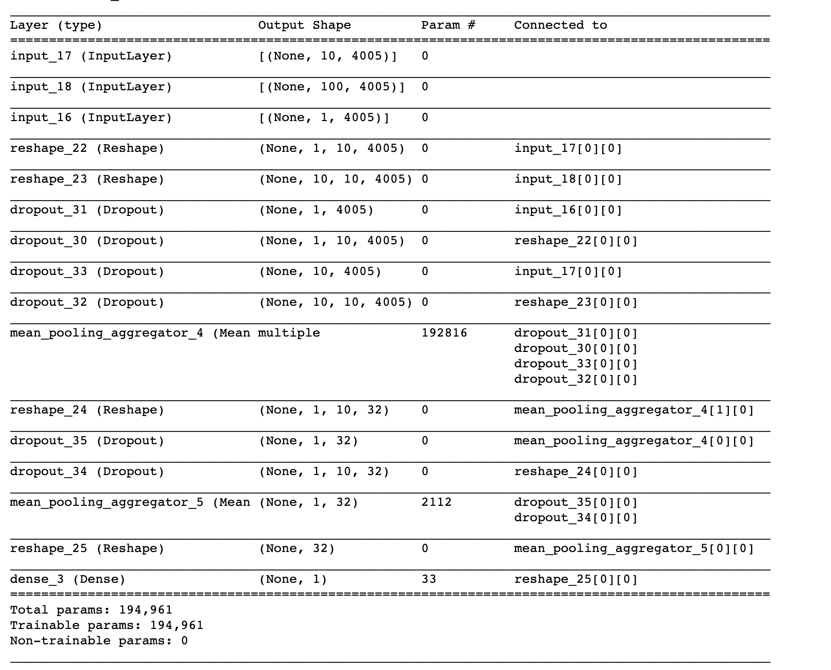
The model is built now, so we can train it and use it for predictions. As you can see, it has 3 inputs and produces a probability score. You can also grab the output of the last Reshape layer to produce the embeddings. Hopefully, you now have a deep understanding of how the model is built, so going forward you can use the stellargraph API to define the same in model in just 5 lines of code.
StellarGraph Model
Using the stellargraph library to build GraphSAGE is quite easy. It has a multitude of parameters, so make sure to study the documentation here. Feel free to experiment with different aggregators, layer numbers, and layer sizes.
# GraphSage tellargraph model
graphsage_model = GraphSAGE(
    layer_sizes=[32, 32],
    generator=generator,
    aggregator=MeanPoolingAggregator,
    bias=True,
    dropout=0.2,
)

# get input and output tensors
x_inp, x_out = graphsage_model.in_out_tensors()
# pass the output tensor through the classification layer
prediction = layers.Dense(1, activation="sigmoid")(x_out)

# build and compile
model = Model(inputs=x_inp, outputs=prediction)
model.compile(
    optimizer=optimizers.Adam(lr=0.005),
    loss=losses.binary_crossentropy,
    metrics=[metrics.AUC(num_thresholds=200, curve='ROC'), 'acc'],
)
model.summary()
For those who have followed the Deep Dive section, these two models should be identical. For those who chose to go to this section straight ahead, you now have built and compiled a GraphSAGE model, so now we can move on to training and predicting.
Training and Evaluation
Training this model is no different to training any other Keras model. We’re providing the generators from above as training and validation datasets but you could easily define the inputs yourself.
cbs = [EarlyStopping(monitor="val_loss", mode="min", patience=2)]
history = model.fit(
    train_gen,
    epochs=100,
    validation_data=val_gen,
    verbose=1,
    shuffle=False,
    callbacks = cbs)
With the model trained, we can evaluate it first on the test set, and then on the holdout dataset.
# Function to evaluate
def evaluate_preds(true, pred):
    auc = roc_auc_score(true, pred)
    pr = average_precision_score(true, pred)
    bin_pred = [1 if p > 0.5 else 0 for p in pred]
    f_score = f1_score(true, bin_pred)
    print('ROC AUC:', auc)
    print('PR AUC:', pr)
    print('F1 score:', f_score)
    print(confusion_matrix(true, bin_pred, normalize='true'))

    return auc, pr, f_score

# make predictions for the test set
test_preds = model.predict(test_gen)

auc, pr, f_score = evaluate_preds(test_labels.values, test_preds.ravel())
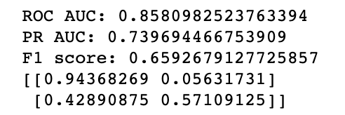
As you can see, the results are pretty good and are just slightly behind the GCN from the previous blog. Now, let’s evaluate the holdout dataset that the model has never seen (GraphSAGE’s unique selling point)
Evaluation on New Nodes
# need to redefine generator to include all the nodes
all_generator = GraphSAGENodeGenerator(G, batch_size, num_samples)

holdout_nodes = targets['ml_target'].index.difference(labels_sampled.index)
holdout_labels = targets['ml_target'][hold_out_nodes]

holdout_generator = all_generator.flow(holdout_nodes)

# making prediction
holdout_preds = model.predict(holdout_generator)

holdout_auc, holdout_pr, holdout_f_score = evaluate_preds(holdout_labels.values, holdout_preds.ravel())
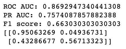
The results for the holdout dataset are about the same as for the test set meaning that GraphSAGE is indeed working. It has learned how to aggregate the neighbours’ features into the node classification prediction, so now, anytime a new node gets added to the graph, we can do the following process:
- Get the features of this node
- Get the features of its 10 neighbours
- Get the features of the neighbours’ neighbours (10 each)
- Pass these 3 matrices through the GraphSAGE model
- Ge the prediction for the new node
Embedding
Finally, we can also check if the embeddings of the holdout nodes make sense, just to sense check the model
# define the model
embedding_model = Model(inputs=[model.layers[2].input, model.layers[0].input, model.layers[1].input],
                        outputs=[model.layers[-3].output]) # output grabs the last reshape layer with shape (None, 32)

# make prediction
holdout_embeddings = embedding_model.predict(holdout_generator)

# UMAP embeddings
m = umap.UMAP()
vis_embs = m.fit_transform(holdout_embeddings)

# plot
sns.scatterplot(x = vis_embs[:, 0], y = vis_embs[:, 1], hue = labels_holdout.values)
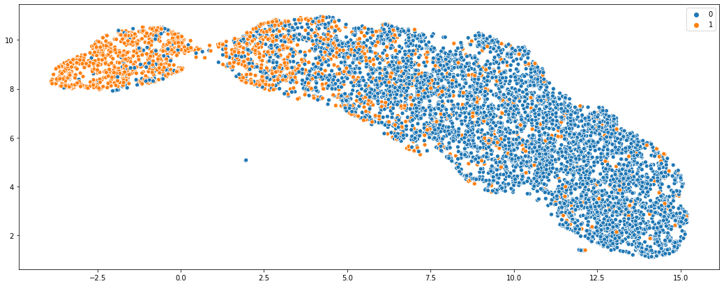
As you can see, while there is some noise, two classes are distinctly separated which what we’d expect.
Conclusion
GraphSAGE network is not only a powerful graph algorithm, but also one of the very few inductive learning approaches suitable for production. I hope that after reading this blog you have a better understanding of GraphSAGE and an intuition of why it works. You also saw how the model is implemented in the stellargraph library and how it can be used for classification.
Thank you for reading, and if you have any questions or comments, feel free to reach out using my email or LinkedIn.
![]()