In the previous blog we saw how the node proximity can be used in classification via label propagation. It was similar to averaging label information from the node neighbours which is quite a naive approach, though effective. There is another way to extract the neighbourhood information from the graph - node embeddings. If you’ve ever worked with NLP, you’ll know what I’m talking about. We want to represent the nodes in the n-dimensional vector form that reflects the neighbourhood and proximity properties of the graph. Sounds like a mouthful, so let’s take a quick look at the example below. You can find all the code in this notebook
Below we’ll do a deep dive into DeepWalk and Node2Vec and a large portion of the code was taken from karateclub’s source code. You can read the package’s documentation, they did a fantastic job implemneting all of these models. Don’t forget to start the github repo as well!
Karate Club Example
We are going to use the famous Zachary’s karate club dataset which comes with NetworkX package and karateclub’s implementation of the DeepWalk algorithm. Each student in the graph belongs to 1 of the 2 karate clubs - Officer or Mr. Hi.
G = nx.karate_club_graph()  # load data

clubs = []  # list to populate with labels
for n in G.nodes:
    c = G.nodes[n]['club']  # karate club name, can be either 'Officer' or 'Mr. Hi'
    clubs.append(1 if c == 'Officer' else 0)

pos = nx.spring_layout(G, seed=42) # To be able to recreate the graph layout
nx.draw_networkx(G, pos=pos, node_color = clubs, cmap='coolwarm') # Plot the graph
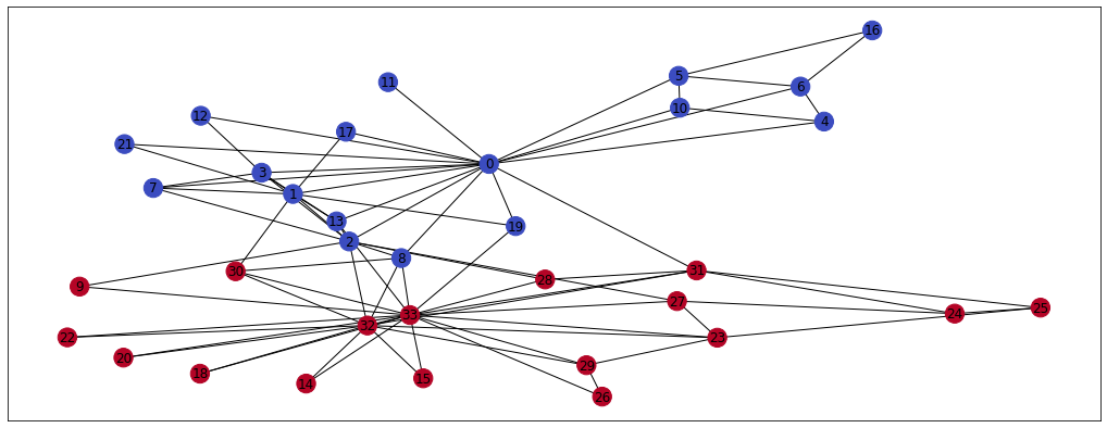
As you can see, members of the karate clubs talk mainly to their club members. Only a few members (nodes) are connected to the opposite coloured nodes. This information could be very valuable for e.g. classification or community detection tasks and we can represent it using the node embeddings. I’m going to use the karateclub’s implementation of DeepWalk now, just to show you how the desired outcome looks like. You can refer to the paper here but we’ll deep dive into the algorithm later in the blog as well.
model = DeepWalk(dimensions=124)  # node embedding algorithm
model.fit(G)  # fit it on the graph
embedding = model.get_embedding()  # extract embeddings

print('Number of karate club members:', len(G.nodes))
print('Embedding array shape:', embedding.shape)
Using DeepWalk (which is a black box algorithm for now) each karate club member is now represented by a vector of size 124. These vectors should reflect the graph neighbourhoods, i.e. the different clubs should be far away from each other. We can check it by reducing the 124 dimensional data into 2 dimensional data using umap-learn package and making a scatter plot.
u = umap.UMAP(random_state=42)
umap_embs = u.fit_transform(embedding)

ax = sns.scatterplot(x = umap_embs[:, 0], y = umap_embs[:, 1], hue = clubs)
a = pd.DataFrame({'x': umap_embs[:, 0], 'y': umap_embs[:, 1], 'val': G.nodes})
for i, point in a.iterrows():
    ax.text(point['x']+.02, point['y'], str(point['val']))
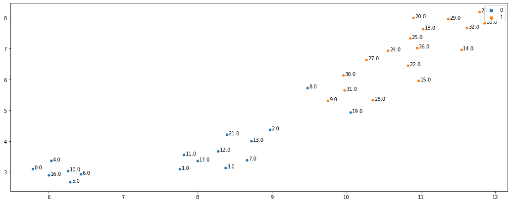
As you can see, the embeddings did very well at representing graph neighbourhoods. Not only are the two karate clubs clearly separated but the members connected to the other clubs are more in the middle (e.g. nodes 28, 30, 8, and 2). In addition, the algorithm seems to have found a sub-community in the “Officer” karate club, which just shows how useful these embeddings can be. To summarise, DeepWalk (and any other neighbourhood based node embedding algorithm) represents the nodes as vectors which capture some neighbourhood information from the graph.
Now that you have an intuitive understanding of what are we trying to achieve on the graph, let’s see how exactly DeepWalk does its magic. To do that, we first need to understand the concept of random walk on graph.
Random Walk
Random walk is a sequence of nodes, where next node is chosen randomly from the adjacent nodes. For example, let’s start our random walk from node 25. From the graph above we can see that the node 25 (right-most) is connected to the nodes 24 and 31. Hence, using a coin-flip we’ll determine where we go next. If we’ve arrived at the node 24, we can see that it’s connected to the members 23, 27, and 31. Again, we need to choose randomly where to go next. This “walk” continues until we’ve reached the desired walk length. Let’s write a simple function to implement this in code.
def random_walk(start_node, walk_length):
    walk = [start_node]  # starting node

    for i in range(walk_length):
        all_neighbours = [n for n in G.neighbors(start_node)]  # get all neighbours of the node
        next_node = np.random.choice(all_neighbours, 1)[0]  # randomly pick 1 neighbour
        walk.append(next_node)  # append this node to the walk
        start_node = next_node  # this random node is now your current state

    return walk

# Example use
walk = random_walk(6, 20)  # random walk from node 6
print('Steps in random walk:', walk)

walk_graph = G.subgraph(walk)
pos = nx.spring_layout(walk_graph, seed=42)
nx.draw_networkx(walk_graph, pos=pos, cmap='coolwarm')

# Generated output for me:
# Steps in random walk: [6, 5, 16, 5, 10, 5, 16, 5, 0, 7, 1, 3, 2, 27, 2, 7, 3, 2, 9, 2, 1]
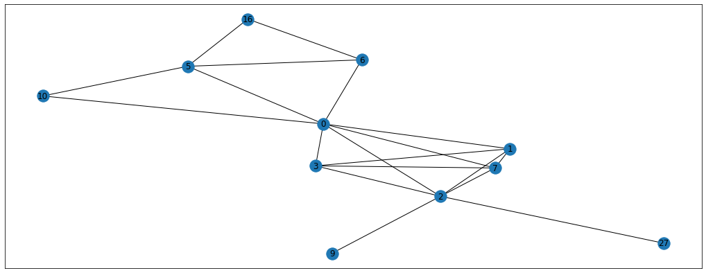
So we’ve generated a random walk with the length of 20 starting at node 6. You can follow the steps of this walk on the graph above and see that every step is located between the connected dots. By doing this walk we’ve got useful information about the context of node 6. By that I mean that we now know some of the neighbours (and neighbours’ neighbours) of node 6 which could be useful in classification problem, for example. By repeating this random walk multiple times for all the nodes in the graph, we can get a bunch of “walk” sequences that contain useful information. The paper suggests doing around 10 walks per node with the walk length of 80. We could implement this with 2 for-loops but, luckily for us, karateclub package has already implemented this for us (and it’s much faster). Here’s how you’d get the random walks in 2 lines of code.
walker = RandomWalker(walk_length = 80, walk_number = 10)
walker.do_walks(G)  # you can access the walks in walker.walks
Skip-Gram
Now the question is - how can we get meaningful embeddings using the generated random walks? Well, if you’ve ever worked with NLP you already know the answer - use the Word2Vec algorithm. In particular, we’re going to use the skip-gram model with a hierarchical softmax layer. There are a lot of detailed resources about the inner workings of these algorithms, but here are my favourites - Word2Vec explained by Rasa and hierarchical softmax explained by Chris McCormick.
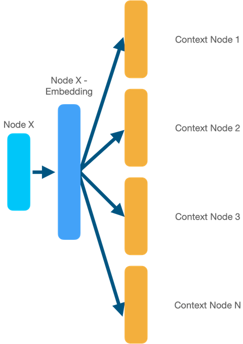
The main idea of the skip-gram model is to predict the context of a sequence from a particular node (or word). For example, if we want to train embeddings for node 6 (example above), we’ll train our model (usually a simple dense neural network) with the goal to predict the nodes that appear in its random walks. So, the model’s input will be the node 6 (one-hot-encoded), middle layer will be the actual embedding, and output will be prediction of the node’s context. This is a very high-level explanation and I encourage you to watch the videos above if you feel confused.
Since it’s the same process as with Word2Vec, we can use the gensim implementation of the algorithm to get the embeddings.
model = Word2Vec(walker.walks,  # previously generated walks
                 hs=1,  # tells the model to use hierarchical softmax
                 sg = 1,  # tells the model to use skip-gram
                 size=128,  # size of the embedding
                 window=5,
                 min_count=1,
                 workers=4,
                 seed=42)

embeddings = model.wv.vectors
print('Shape of embedding matrix:', embeddings.shape)
And that’s it! The embeddings are trained, so you can use them e.g. as features for your supervised model or to find clusters in your dataset. Let’s now see how we can use DeepWalk on real classification tasks.
Facebook Data
Facebook data can be downloaded from the dataset repo. This particular dataset is a network of Facebook Pages and was used in this paper. As in the previous blog, there are 3 files - edges, targets, and features.
edges_path = 'datasets-master/facebook_large/facebook_edges.csv'
targets_path = 'datasets-master/facebook_large/facebook_target.csv'
features_path = 'datasets-master/facebook_large/facebook_features.json'

#Read in edges
edges = pd.read_csv(edges_path)

#Read in targets
targets = pd.read_csv(targets_path)
targets.index = targets.id


# Read in features
with open(features_path) as json_data:
    features = json.load(json_data)

max_feature = np.max([v for v_list in features.values() for v in v_list])
features_matrix = np.zeros(shape = (len(list(features.keys())), max_feature+1))

i = 0
for k, vs in tqdm(features.items()):
    for v in vs:
        features_matrix[i, v] = 1
    i+=1
With data read in, we can now build a graph and generate the embeddings.
DeepWalk on Facebok Graph
# Read in Graph
graph = nx.convert_matrix.from_pandas_edgelist(edges, "id_1", "id_2")

# Do random walks
walker = RandomWalker(walk_length = 80, walk_number = 10)
walker.do_walks(graph)

# Train Skip-Gram model
model = Word2Vec(walker.walks,  # previously generated walks
                 hs=1,  # tells the model to use hierarchical softmax
                 sg = 1,  # tells the model to use skip-gram
                 size=128,  # size of the embedding
                 window=10,
                 min_count=1,
                 iter = 1,
                 workers=4,
                 seed=42)
DeepWalk model is trained, so we can use the embeddings for classification. We can quickly sense check the model by looking at the nearest neighbours in the embeddings space of some of the Facebook’s pages. For example, let’s check the most similar nodes to the Facebook page of American Express (ID 22196) and the BBC’s show Apprentice (ID 451)
similar_to = '22196'
targets.loc[[int(similar_to)] + [int(v[0]) for v in model.wv.most_similar(similar_to)], :].head()
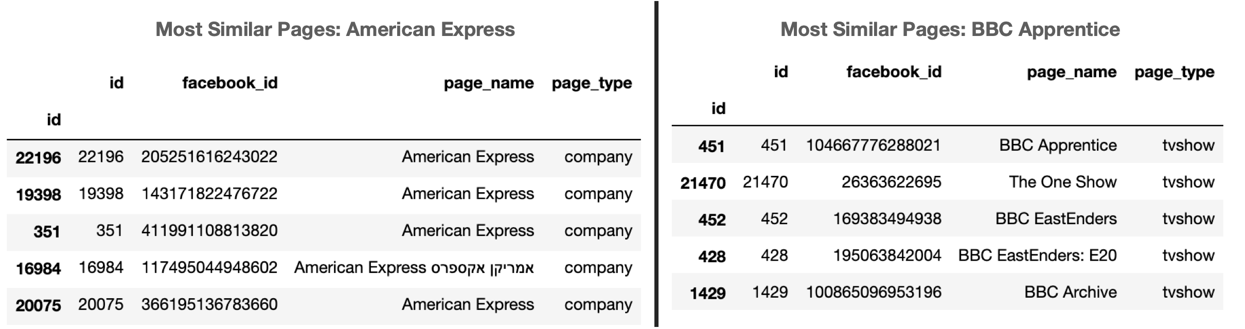
As you can see, the nearest neighbours are incredibly similar to the original pages and all of this is achieved without even knowing what the original pages are about! Hence, the embeddings that the DeepWalk has learned are meaningful and we can use them in the classifier. We can build a simple Random Forest model to see what performance we can achieve purely using the embeddings.
# Get targets
y = targets.loc[[int(i) for i in list(features.keys())], 'page_type']

# Get corresponding embeddings
X_dw = []
for i in y.index:
    X_dw.append(model.wv.__getitem__(str(i)))

# Train/test split
X_train, X_test, y_train, y_test = train_test_split(X_dw, y, test_size=0.2)

# Train RF model
rf = RandomForestClassifier()
rf.fit(X_train, y_train)
y_pred = rf.predict(X_test)

# Evaluate
print(f1_score(y_test, y_pred, average='micro'))
print(confusion_matrix(y_test, y_pred, normalize='true'))

#F1 Score: ~ 0.93
As you can see, the performance is really good with F1 score of ~0.93 (yours will be different but should still be high). We can try to improve the performance a bit further by using a different sampling strategy in random walk that was described in Node2Vec algorithm paper.
Node2Vec on Facebook Graph
Node2Vec is very similar to DeepWalk, but the random walks are generated a bit differently. Recall that in the pure random walk, neighbourhood nodes have an equal probability to be chosen as next step. Here instead, we have 2 hyperparameters to tune - p and q. p and q control how fast the walk explores and leaves the neighbourhood of the starting node u.
- p - high value means that we’re less likely to return to the previous node
- q - high value approximates the Breadth-First-Search meaning that the neighbourhood around the node is explored. Low values give higher chance to go outside the neighbourhood and hence approximates the Depth-First-Search
Here’s the code block from karate-club package that does the Biased Random Walk. I’m showing it here so that you have a better understanding of what’s happening under the hood.
def biased_walk(start_node, walk_length, p, q):
    walk = [start_node]
    previous_node = None
    previous_node_neighbors = []
    for _ in range(walk_length-1):
        current_node = walk[-1]  # currnet node ID
        current_node_neighbors = np.array(list(graph.neighbors(current_node)))  # negihbours of this node
        probability = np.array([1/q] * len(current_node_neighbors), dtype=float)  # outwards probability weight determined by q
        probability[current_node_neighbors==previous_node] = 1/p  # probability of return determined by p
        probability[(np.isin(current_node_neighbors, previous_node_neighbors))] = 1  # weight of 1 to all the neighbours which are connected to the previous node as well
        norm_probability = probability/sum(probability)  # normalize the probablity
        selected = np.random.choice(current_node_neighbors, 1, p=norm_probability)[0]  # select the node from neighbours according to the probabilities from above
        walk.append(selected)  # append to the walk and continue
        previous_node_neighbors = current_node_neighbors
        previous_node = current_node

    return walk
Let’s compare 2 extreme scenarios:
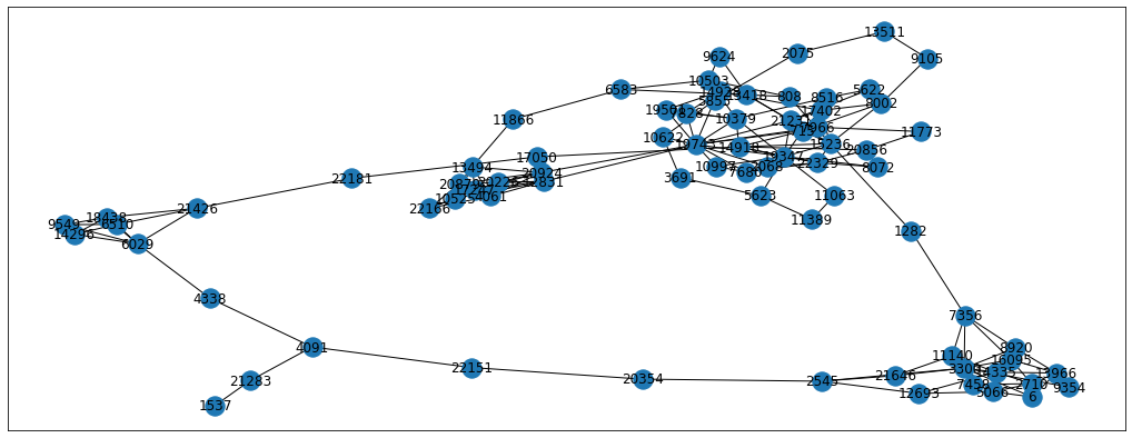
- p = 10, q = 0.1 - here we expect the random walk to go outwards and explore the adjacent clusters as well
- p = 0.1, q = 10 - here we expect the random walk to stay very local and explore the neighbourhood around the starting node
p = 10
q = 0.1
walk = biased_walk(6, 80, p, q)
# Visualise the subgraph
subgraph_nodes = list(nx.dfs_preorder_nodes(graph, 7))
G = graph.subgraph(walk)
pos = nx.spring_layout(G, seed=42)
nx.draw_networkx(G, pos=pos, cmap='coolwarm')
p = 0.1
q = 10
walk = biased_walk(6, 80, p, q)
# Visualise the subgraph
subgraph_nodes = list(nx.dfs_preorder_nodes(graph, 7))
G = graph.subgraph(walk)
pos = nx.spring_layout(G, seed=42)
nx.draw_networkx(G, pos=pos, cmap='coolwarm')
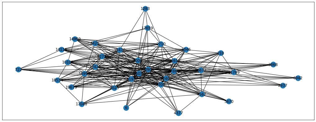
From the images we can see the differences between the resulting random walks. Each problem will have its own perfect p and q parameters so we can treat them as hyperparameters to tune. For now, let’s just set the parameters to p=0.5 and q=0.25 but feel free to experiment with other parameters as well. Also, we’re going to use the karate-club implementation of BiasedRandomWalker for the simplicity sake. Please note that biased sampling takes longer to calculate, so grid searching the optimal hyperparameters is a long procedure.
# Biased random walks
b_walker = BiasedRandomWalker(80, 10, 0.5, 0.25)
b_walker.do_walks(graph)

# Train skipgram
node_vec = Word2Vec(b_walker.walks,  # previously generated walks
                 hs=1,  # tells the model to use hierarchical softmax
                 sg = 1,  # tells the model to use skip-gram
                 size=128,  # size of the embedding
                 window=10,
                 min_count=1,
                 iter = 1,
                 workers=4,
                 seed=42)

# Get corresponding Node2Vec embeddings
X_node_vec = []
for i in y.index:
    X_node_vec.append(node_vec.wv.__getitem__(str(i)))

# Train/test split
X_train, X_test, y_train, y_test = train_test_split(X_node_vec, y, test_size=0.2) # train/test split

# Train RF
rf = RandomForestClassifier()
rf.fit(X_train, y_train)
y_pred = rf.predict(X_test)

print(f1_score(y_test, y_pred, average='micro'))
print(confusion_matrix(y_test, y_pred, normalize='true'))

#F1 Score: ~0.93
As we can see, the results are roughly the same, so we’d need to do a proper grid-search to find the parameters that would increase the accuracy. We can also use UMAP to plot these embeddings, and see if the embeddings differ in some way.
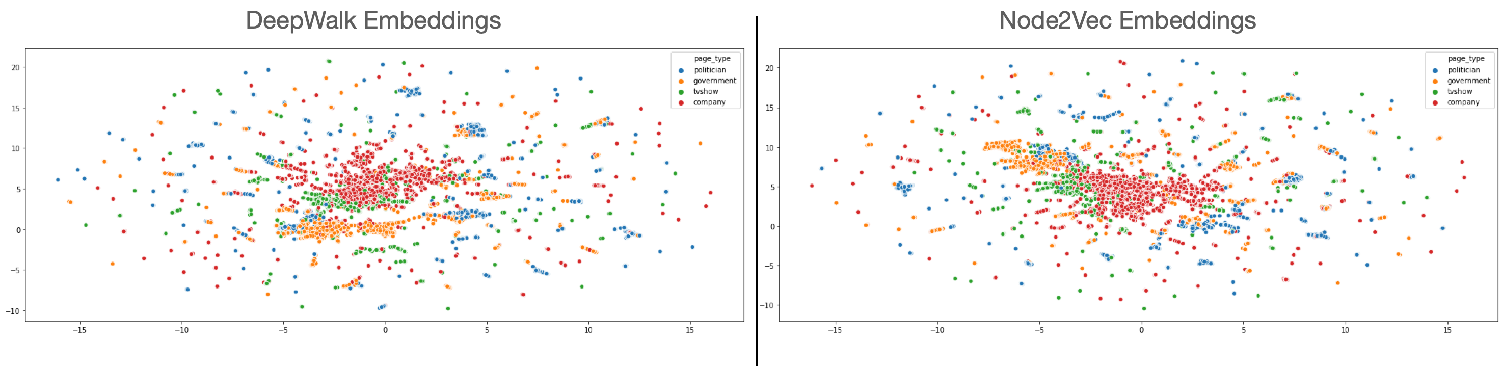
As can be seen from the embeddings, the company, government, and tvshows are represented by clear clusters whereas politician clusters are scattered around. Plus, there are pages which are not clustered meaning that they are probably much harder to classify.
Conclusion
Just by using node proximity information from graph we were able to extract node embeddings which were incredibly useful in the downstream task of classification. Here you saw two node embedding algorithms - DeepWalk and Node2Vec. I hope that now you have a better understanding of how these algorithms work, and how to apply them to the real-world graph datasets. Plus, we’ve covered a very important fundamental aspect of random walk, and its variant - biased random walk. These concepts are crucial in working with graphs data and you will encounter them in a lot of other papers. In the next blogs we’ll keep exploring new graph ML algorithms, so stay tuned.