Modelling Customer Lifetime Value

Customer Lifetime Value (CLV) is probably the most useful metric you can have about your customer, yet it’s frequently misunderstood. Let’s clarify the confusion from the beginning - CLV refers to the monetary value of your relationship with a customer, based on the discounted value of future transactions that the customer is going to have. If we phrase the definition this way, it becomes clear that it actually needs a predictive element in it to be accurate. If we know how much profit a customer is going to generate in the future, we can frame our relationship with him accordingly. We can focus our marketing efforts on those who need persuasion or are about to churn, and we can focus on providing the best customer service to the customers with highest value. Most importantly, however, knowing the CLV allows us to focus on the long-term results, not the short-term profits. This blog will show you exactly how you can make a predictive CLV model.

Intuition

It’s crucial to understand the intuition behind CLV. These are the main assumptions that we make:

1. At each point in time, a customer can decide to buy
2. Probability of buying is unique for each user and it depends on the historical behaviour
3. Each customer can churn after a transaction
4. Probability of churn is unique for each user and it depends on the historical behaviour

As you can see, we have essentially 2 functions that we need to model - probability of buy at time t, and probability of churn at time. Consider the figure below:

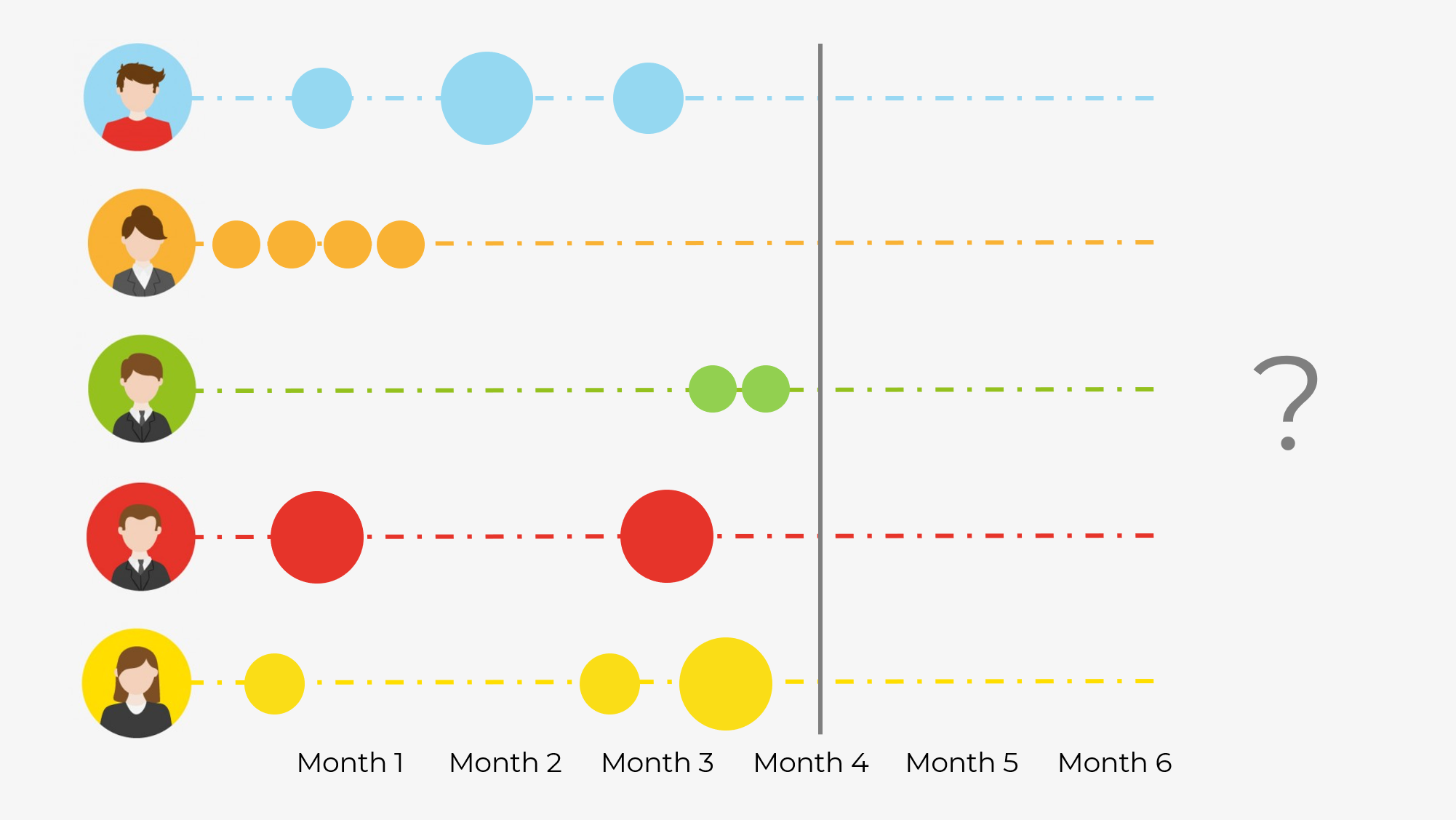
Who do you think is the most valuable customer here? The answer here could be different, but it’s definitely not the Orange customer. Just from the purchasing behaviour we can see that she has made a sequence of rapid purchases and has never returned. Hence, we can conclude that she has likely churned, and her lifetime value is close to zero. The customer Green however, just recently became our customer and his pattern tells us that he might continue shopping at our store. Hence his CLV is higher, even though he has spent less money with us than Orange. Let’s find out how can we model this type of reasoning in Python.

Prep

To model the CLV you need to have transaction data. I took the data for this blog from a Kaggle competition called “Acquire Valued Shoppers”. The disavantage of this dataset is that it’s huge (about 20GB), so I’ve extracted transactions for a single store (which still amounts for 700MB). You can find the entire notebook in my github repo as always. As a main package, I’ll be using lifetimes - a Python package that has APIs for the models that we’re about to use, plus some amazing utility functions. You can simply pip install lifetimes and it should work out-of-the-box. Please, check their documentation if you need more in-depth explanation of algorithms or if you want to see other methods that they offer.

Data Preprocessing

Once you have acquired your data in the transactions format, make sure that it has the following columns - customer ID, date of the transaction, and revenue that it has generated. From these 3 columns we can convert the data into RFM format - Recency, Frequency, and Monetary Value.

1. Recency - it’s the number of time periods between their last and first purchases. In other words, it shows how much time has this customer been active.
2. Frequency - counts the number of time-periods where you had a repeat purchase.
3. Monetary value - is the average spend by a customer per repeat purchase day. Another column that we need is T, which is the number of time periods that the customer is listed in your transactions dataset.

In addition to transforming the data into RFM, I’ll also split it into train and test sets to ensure that I can get an unbiased estimate of the model’s quality. Because the CLV (actually Residual CLV) is time-dependent, the train/test split is different than in other ML tasks. Here, we’re going to take the first 8 months as training dataset, and the remaining 4 months will serve as the holdout dataset. Luckily, there’s a utility function in lifetimes package, so splitting the data is quite easy.

#Import 
df = pd.read_csv('./transactions_103338333.csv', parse_dates = ['date'])

#Select 1 year of data with positive sales (no refunds)
df_year = df.loc[(df.date <= '2013-03-02') & (df.purchaseamount > 0), ['id', 'date', 'purchasequantity', 'purchaseamount']]

#RFM
#Split
rfm_train_test = calibration_and_holdout_data(df_year, 'id', 'date',
                                        calibration_period_end='2012-11-01',
                                        observation_period_end='2013-03-02',
                                                  monetary_value_col = 'purchaseamount')


#Filter out negatives
rfm_train_test = rfm_train_test.loc[rfm_train_test.frequency_cal > 0, :]

rfm_train_test.head()

This is what the transformed data should look like. As you can see, each customer ID has a row with train and test columns in the dataset.

Now, with data in the right format, we’re ready to go to the modelling section.

Modelling & Evaluation

The modelling & evaluation process is going to be the following:

1. Fit and evaluate BG/NBD model for frequency prediction
2. Fit and evaluate Gamma-Gamma model for monetary value prediction
3. Combine 2 models into CLV model and compare to baseline
4. Refit the model on the entire dataset

1. BG/NBD Model

This model is an industry standard when it comes to purchase frequency modelling. It stands for Beta Geometric/Negative Binomial Distribution and was introduced by Fader et al. (2005). Its basic idea is that sales of each customer can be described as a combination of his/her probability to buy and to churn. As such, it models the sales for a particular customer as a function of 2 distributions - Gamma for transactions and probability of churn as Beta. The model that we’re about to fit learns 4 parameters that are able to describe these distributions. In this way, we get a unique transaction and churn probability for each customer (as we want) without having a model with hundreds of parameters.

lifetimes somewhat follows the sklearn syntaxis, so fitting and predicting is quite familiar. Remember, we fit on the training columns (with suffix ‘_cal’) and we’re predicting for the testing period.

#Train the BG/NBD model
bgf = BetaGeoFitter(penalizer_coef=0.0)
bgf.fit(rfm_train_test['frequency_cal'], rfm_train_test['recency_cal'], rfm_train_test['T_cal'])

#Predict
predicted_bgf = bgf.predict((datetime.datetime(2013, 3, 2)- datetime.datetime(2012, 11, 1)).days, #how many days to predict
                        rfm_train_test['frequency_cal'], 
                        rfm_train_test['recency_cal'], 
                        rfm_train_test['T_cal'])

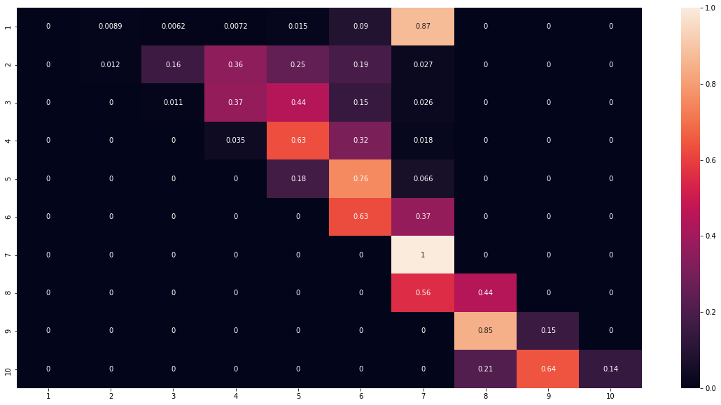
Now it’s time to compare the predicted purchase frequency with the actual target data (it’s in the column ‘frequency_holdout’). I’m going to make a quantitative comparison by looking at the Mean Absolute Error (MAE), but I’ll also do the scatter plot to qualitatively see if a model is any good. In addition, I’m going to bin the frequencies into 10 bins, so that I can calculate the F1 score and plot a confusion matrix. Here’s the code to do that:

actual = rfm_train_test['frequency_holdout']
predicted = predicted_bgf

def evaluate_clv(actual, predicted, bins):
    print(f"Average absolute error: {mean_absolute_error(actual, predicted)}")
    #Evaluate numeric
    plt.figure(figsize=(10, 7))
    plt.scatter(predicted, actual)
    plt.xlabel('Predicted')
    plt.ylabel('Actual')
    plt.title('Predicted vs Actual')
    plt.show()
    
    #Evaluate Bins
    est = KBinsDiscretizer(n_bins=bins, encode='ordinal', strategy='kmeans')
    est.fit(np.array(actual).reshape(-1, 1))
    actual_bin = est.transform(np.array(actual).reshape(-1, 1)).ravel()
    predicted_bin = est.transform(np.array(predicted).reshape(-1, 1)).ravel()
    
    cm = confusion_matrix(actual_bin, predicted_bin, normalize='true')
    df_cm = pd.DataFrame(cm, index = range(1, bins+1),
                      columns = range(1, bins+1))
    plt.figure(figsize = (20,10))
    sns.heatmap(df_cm, annot=True)

    # fix for mpl bug that cuts off top/bottom of seaborn viz
    b, t = plt.ylim() # discover the values for bottom and top
    b += 0.5 # Add 0.5 to the bottom
    t -= 0.5 # Subtract 0.5 from the top
    plt.ylim(b, t) # update the ylim(bottom, top) values
    plt.show()
    print(f'F1 score: {f1_score(actual_bin, predicted_bin, average="macro")}')
    print('Samples in each bin: \n')
    print(pd.Series(actual_bin).value_counts())

evaluate_clv(actual, predicted, bins=10)

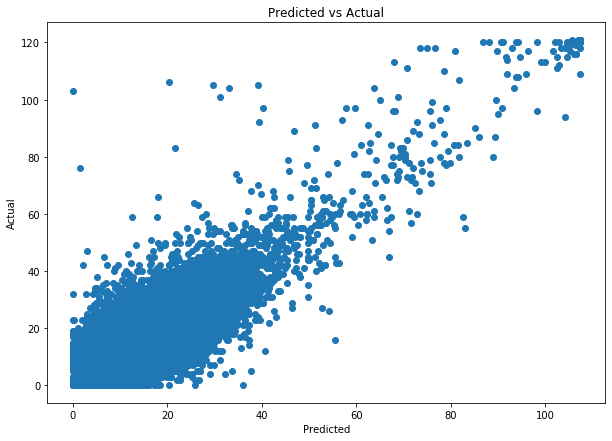
The resulting average absolute error is ~ 2.92 which is quite good for such a simple model. In addition, by looking at the scatterplot output, we can see that the model’s predictions are indeed quite accurate.

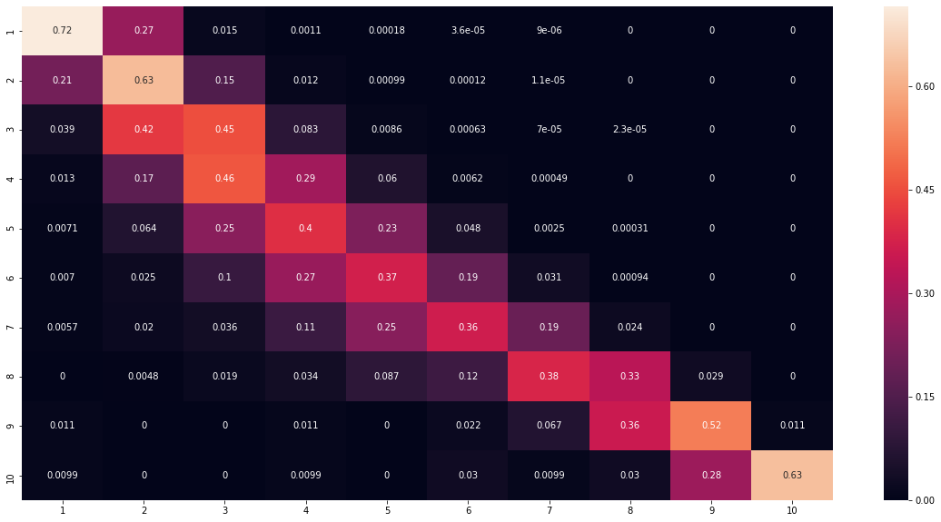
Looking at binned results, we see quite an average F1 score of 0.46. Nevertheless, when we look at the confusion matrix, we can see that the model does get the bins correctly with a margin or error of ~ 1 bin.

Now that we’ve validated the BG/NDB model, let’s move on to Gamma-Gamma model.

2. Gamma-Gamma Model

Gamma-Gamma model presented in the same paper, adds a monetary value into the mix. It does so by assuming that the spend of an individual is right-skewed and follows a Gamma distribution. One of the parameters required to describe Gamma distribution, also varies per customer (so each customer again ends up with different propensity to spend) and it also follows a Gamma distribution. That’s why the model is called Gamma-Gamma.

To ensure that we can use Gamma Gamma, we need to check if frequency and monetary values are not correlated. Running rfm_train_test[['monetary_value_cal', 'frequency_cal']].corr() will confirm that the two arrays are very weakly correlated with correlation coefficient of only 0.14. Hence, we can fit and evaluate the Gamma-Gamma model:

#Model fit
ggf = GammaGammaFitter(penalizer_coef = 0)
ggf.fit(rfm_train_test['frequency_cal'],
        rfm_train_test['monetary_value_cal'])

#Prediction
monetary_pred = ggf.conditional_expected_average_profit(rfm_train_test['frequency_holdout'],
                                        rfm_train_test['monetary_value_holdout'])

#Evaluation
evaluate_clv(rfm_train_test['monetary_value_holdout'], monetary_pred, bins=10)

The average error is quite small, only 1.09 but the F1 score is quite bad - only 0.2. This is due to the way that the purchases get modelled - Gamma-Gamma is too simplistic to capture most of the variation in data. However, when we look at the scatter plot we can see that the predictions are still fairly good:

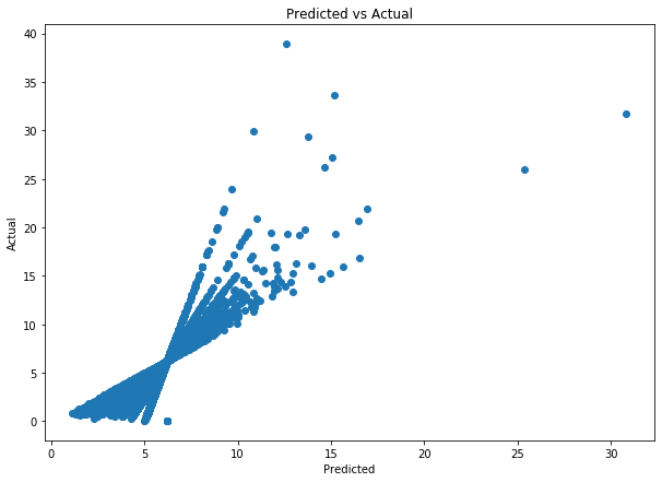
Furthermore, when we look at the confusion matrix, we can see that larger values are being placed to the higher bins, which is already great. Keep in mind, that this model will only augment the BG/NBD by providing the average order value, not replace it. Now that 2 models are validated and fitted, we can combine both of them into a complete CLV model.

3. CLV Model

This model will take the prediction of expected purchase and it will combine it with the expected purchase value. Together with the discount rate, these components allow us to arrive at an estimate of how much a customer is worth to you in a given period of time (e.g. here it’s 4 months).

clv = ggf.customer_lifetime_value(
    bgf, #the model to use to predict the number of future transactions
    rfm_train_test['frequency_cal'],
    rfm_train_test['recency_cal'],
    rfm_train_test['T_cal'],
    rfm_train_test['monetary_value_cal'],
    time=4, # months
    discount_rate=0.01 # monthly discount rate ~ 12.7% annually
)

#Assign the clv values
rfm_train_test['clv'] = clv

To somehow evaluate the performance of this model, I’m going to compare it to a simple baseline. Let’s imagine a scenario - we need to pick top 20% of our best users to target. Those who are not targeted will not purchase anything, so we need to be careful in the selection process. One way to do it, would be to select those users who have previously purchased a lot. I’ll call this method a naive approach and I’ll compare it to the model approach. It turns our that if I pick 20% of users according to their historic purchase frequency, I’ll end up with 68,818 transactions less in the validation period than if I had picked 20% according to the highest predicted CLV. You can check the code by following the link in the beginning.

We can now do the same for revenue. If we’ve picked our top 20% according to their modelled CLV, we end up with additional 1,532,938 compared to the naive approach of picking top 20% according to their historic monetary value. This additional revenue can be visualised in the following graph:

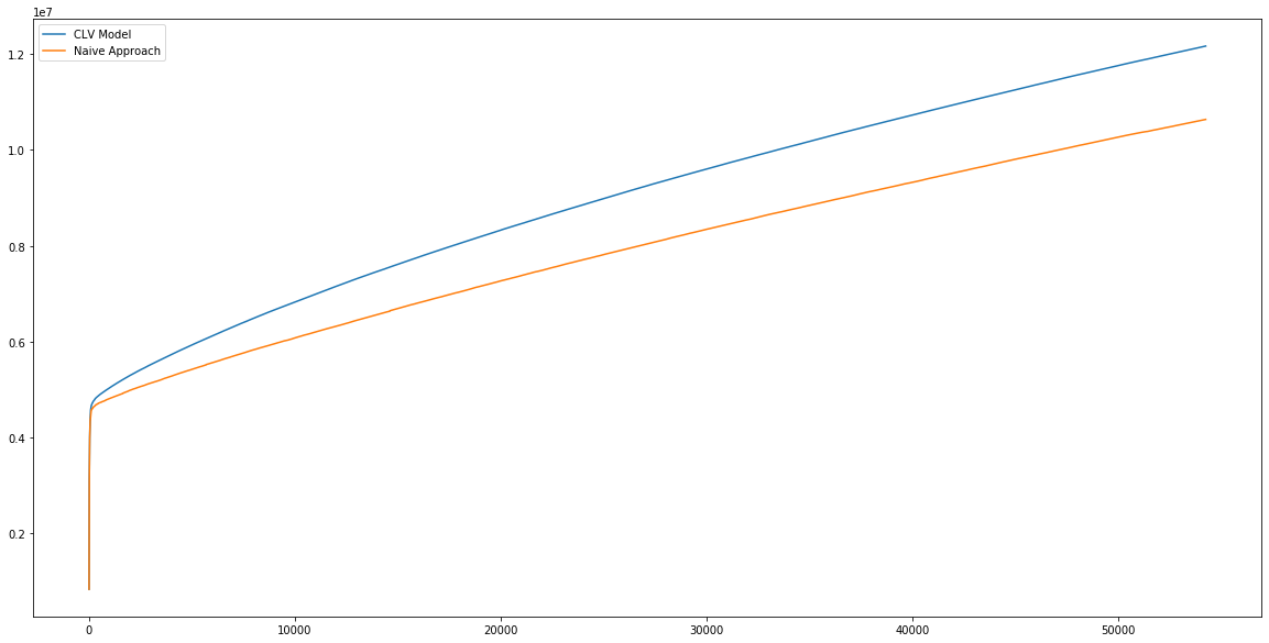
The additional revenue generated is the difference between these two curves. Now that we know that our model does a pretty good job, we can retrain the model on the entire year.

Retraining the Model

This step just follow everything discussed previously to fit a single model in a single script.

#RFM
rfm = summary_data_from_transaction_data(df_year, 'id', 'date', monetary_value_col = 'purchaseamount')
rfm = rfm.loc[rfm.frequency > 0, :]

#BG/NBD
bgf = BetaGeoFitter(penalizer_coef=0.0)
bgf.fit(rfm['frequency'], rfm['recency'], rfm['T'])

#GG
ggf = GammaGammaFitter(penalizer_coef = 0)
ggf.fit(rfm['frequency'],
        rfm['monetary_value'])

#CLV model
clv = ggf.customer_lifetime_value(
    bgf, #the model to use to predict the number of future transactions
    rfm['frequency'],
    rfm['recency'],
    rfm['T'],
    rfm['monetary_value'],
    time=4, # months
    discount_rate=0.01 # monthly discount rate ~ 12.7% annually
)

rfm['clv'] = clv

#Print the top 10 most valued customers
rfm.sort_values('clv', ascending=False).head(10)

So, finally we can see the top 10 most valued customers:

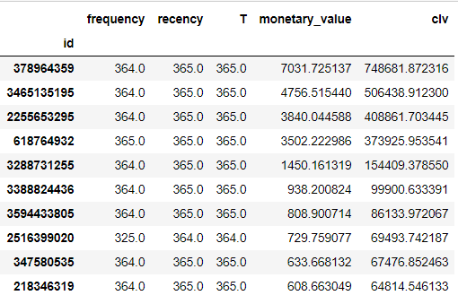
As expected, these are some of the most loyal customers who have been present and buying for the entire year. Well, now you know their IDs. Not bad, right?

Conclusion

To conclude, we’ve just predicted the CLV for the next 4 months for the existing customers. This model jointly models the probability to churn, purchase, and the average purchase value. It’s simple, effective, and quite accurate when we look at the aggregated level. There’s a multitude of applications for the newly predicted CLV - segmenting, ranking, profiling, personalising, etc. Knowing who your best customers are or who is about to churn is quite useful, and we’ve just done it with a few lines of code!

Because this model is quite simple, it also has a few notable limitation. It has high bias as it makes a lot of assumptions about the data. Hence, it probably underfits the data and has inferior predictive performance compared to the more complex Machine Learning models. Also, it cannot take context data (e.g. demographics) into account which, again, limits the predictive power of the model.