In the previous blog, I’ve talked about estimating the Customer Lifetime Value (CLV) using more classical statistical models BG/NBD and Gamma-Gamma. They are simple (only a few parameters to train) yet highly effective in estimating the future purchasing behaviour. Yet, a common question after using these models is - how can I include contextual data, such as demographics, into my CLV model? Well, with BG/NBD you can’t really do it because the model takes no input other than RFM. Luckily, other Machine Learning (ML) algorithms can be easily used to estimate CLV, and they do need as much relevant information as possible about your customers. So, in this blog I’m going to show you how you can approach CLV prediction as ML task, and I’m going to use Deep Neural Networks (DNN) to make a predictive model.
Statistical vs Machine Learning Approach
CLV prediction involves estimating how much money will a particular customers spend in a given period. With statistical models, we saw that we can split customers’ purchasing history into two periods - calibration and holdout. For the sake of consistency, from now on I’m going to refer to the calibration period as features period and holdout period as target period. Here’s the difference between the setups for statistical and ML model fitting:
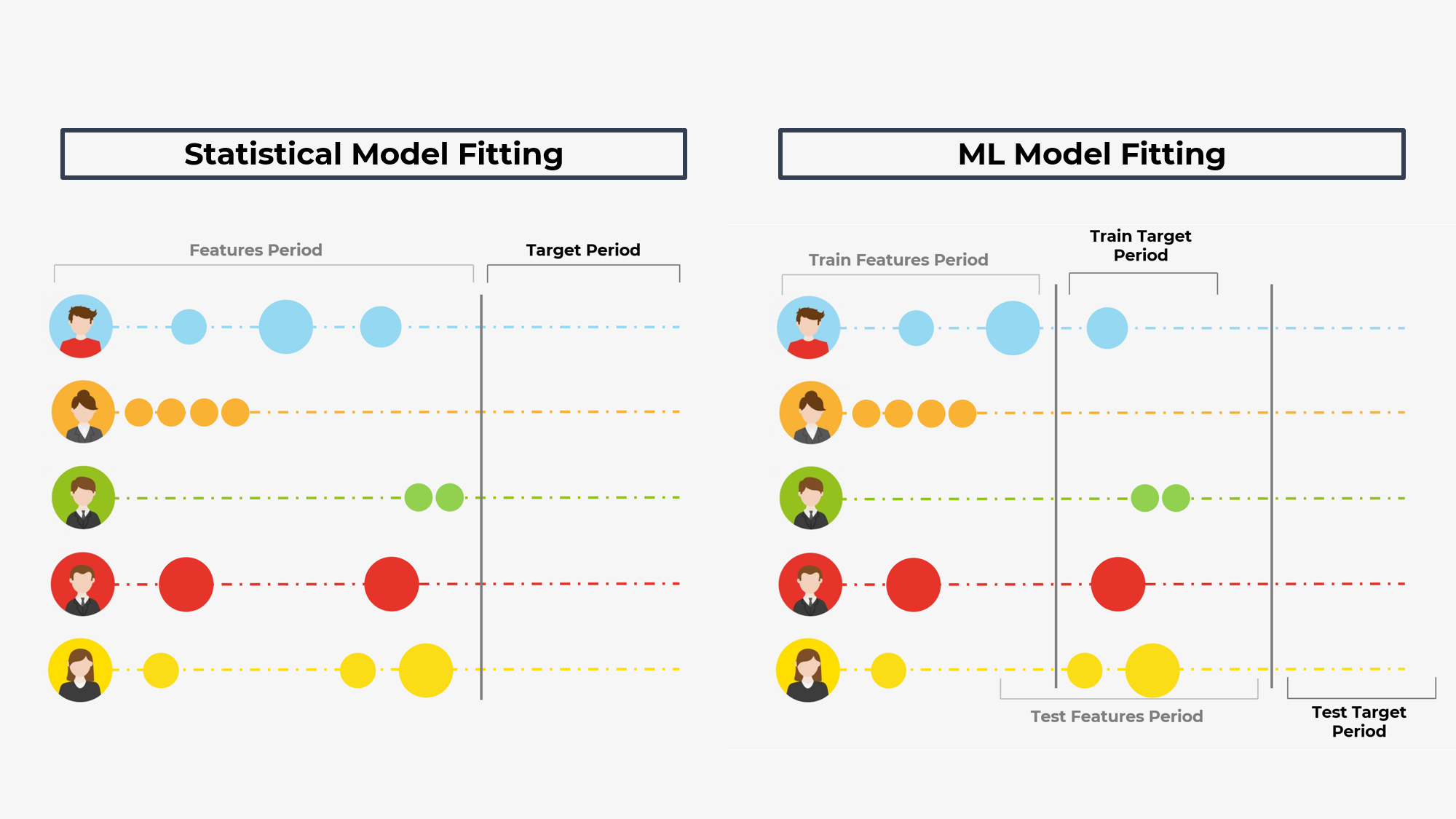
Notice that we don’t need to separate the data into a classical train/test time split for statistical models. This is because models like BG/NBD are estimating latent variables using the features period. In other words, we can see this type of modelling as unsupervised and our features periods is both X and Y of our model. This is not the case for supervised ML algorithms like DNN that we’re going to use. It needs to have some value that it is trained to predict, and we also need to have a subset of these Y values that the model has never seen before to evaluate the performance. As you can see, the ML setup has a training phase (the top timeline) and the testing phase (the bottom timeline). It’s important to keep the date ranges consistent, to ensure that the distribution of data stays the same. Also, this structure clearly shows that the process of estimating the CLV is continuous as any additional purchase may change the forecast. You might be wondering when you should use each approach? As always, the answer is it depends. Nevertheless, here are some signs that one approach may be preferred over another:
Statistical models are good when:
- You have enough repeat purchases for each customer
- You have no access to CRM, website, and other types of context data
- Your dataset is relatively small (~ 1 year of data)
ML models are good when:
- You have a lot of data (> 1 year of data, > 5,000 customers)
- You have access and want to include CRM, website and other context data
As you’ll see, the dataset that we’ll be working with is not really suited for the ML approach, but we’ll proceed anyways since my goal here is to show how to approach CLV problems as regression tasks. Let’s begin!
Prep
You can find the notebook to follow along in my github repo. The data we’re going to be working with is of the online retailer and you can download it from the UCI Machine Learning Repository. Two main modelling packages are lifetimes and tensorflow, so make sure install them as well. Here are all of the imports you’ll need
import pandas as pd
import numpy as np
from datetime import datetime

#Statistical LTV
from lifetimes import BetaGeoFitter, GammaGammaFitter
from lifetimes.utils import calibration_and_holdout_data, summary_data_from_transaction_data

#ML Approach to LTV
import tensorflow as tf
from tensorflow import keras
from tensorflow.keras import layers

#Evaluation
from sklearn.metrics import r2_score
from sklearn.metrics import mean_absolute_error

#Plotting
import matplotlib.pyplot as plt
import seaborn as sns
Data Preprocessing
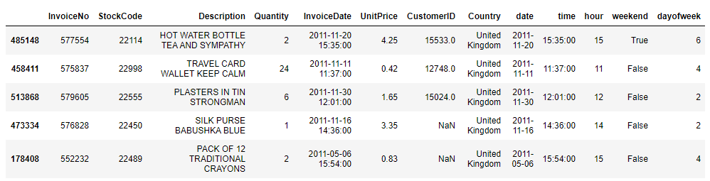
First, let’s read in the data and see how it looks like. Since this is sales data, we should be able to aggregate by date to see the total sales. This will allow us to infer whether there were some structural changes to the data, and what type of pre-processing it needs. Its a useful exercise that I always do and has helped me quite a few times.
#Read in
data = pd.read_csv('CLV_raw.csv', engine='python')
data['InvoiceDate'] = pd.to_datetime(data.InvoiceDate, format = '%d/%m/%Y %H:%M')

#Datetime transformation
data['date'] = pd.to_datetime(data.InvoiceDate.dt.date)
data['time'] = data.InvoiceDate.dt.time
data['hour'] = data['time'].apply(lambda x: x.hour)
data['weekend'] = data['date'].apply(lambda x: x.weekday() in [5, 6])
data['dayofweek'] = data['date'].apply(lambda x: x.dayofweek)
#Get revenue column
data['Revenue'] = data['Quantity'] * data['UnitPrice']

print(data.sample(5))

#Plots a timeseries of total sales
data.groupby('date')['Quantity'].sum().plot()
#Prints the total number of days between start and end
print(data['date'].max() - data['date'].min())
Here’s how the data looks like:
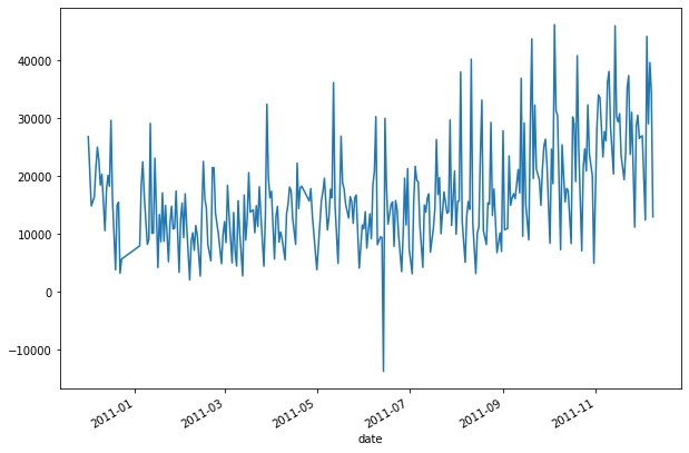
So, we have around 1 year of data. Because the ML approach requires time periods for feature creation, training targets, and validation targets, I’ll split it into the following segments:
- Training Features Period - from 2011-01-01 until 2011-06-11
- Training Target Period - from 2011-06-12 until 2011-09-09
- Testing Features Period - from 2011-04-02 until 2011-09-10
- Testing Target Period - from 2011-09-11 until 2011-12-09
Hence, I’ll be using 161 days to create features. These features will be used to forecast the next 89 days of customer sales. This choice is, of course, quite arbitrary and can be treated as hyperparameter to tune. In general though, you want to have target period that’s about half of your training period. With this information, we can move on to the feature engineering part for the DNN model.
Feature Engineering
The possibility to include additional features into the model besides the RFM is the greatest advantage of this approach. However, it’s also the main limitation as your model is going to be only as good as your features. So, make sure to spend a lot of time on this section, and experiment yourself to find the best features. Here, I’m mainly going to focus on the transactional features as they form a good predictive basis for the future transactional behaviour. Most of them were inspired by this Google post.
def get_features(data, feature_start, feature_end, target_start, target_end):
    """
    Function that outputs the features and targets on the user-level.
    Inputs:
        * data - a dataframe with raw data
        * feature_start - a string start date of feature period
        * feature_end - a  string end date of feature period
        * target_start - a  string start date of target period
        * target_end - a  string end date of target period
    """
    #Double check the periods length
    features_data = data.loc[(data.date >= feature_start) & (data.date <= feature_end), :]
    print(f'Using data from {(pd.to_datetime(feature_end) - pd.to_datetime(feature_start)).days} days')
    print(f'To predict {(pd.to_datetime(target_end) - pd.to_datetime(target_start)).days} days')

    #Transactions data features
    total_rev = features_data.groupby('CustomerID')['Revenue'].sum().rename('total_revenue')
    recency = (features_data.groupby('CustomerID')['date'].max() - features_data.groupby('CustomerID')['date'].min()).apply(lambda x: x.days).rename('recency')
    frequency = features_data.groupby('CustomerID')['InvoiceNo'].count().rename('frequency')
    t = features_data.groupby('CustomerID')['date'].min().apply(lambda x: (datetime(2011, 6, 11) - x).days).rename('t')
    time_between = (t / frequency).rename('time_between')
    avg_basket_value = (total_rev / frequency).rename('avg_basket_value')
    avg_basket_size = (features_data.groupby('CustomerID')['Quantity'].sum() / frequency).rename('avg_basket_Size')
    returns = features_data.loc[features_data['Revenue'] < 0, :].groupby('CustomerID')['InvoiceNo'].count().rename('num_returns')
    hour = features_data.groupby('CustomerID')['hour'].median().rename('purchase_hour_med')
    dow = features_data.groupby('CustomerID')['dayofweek'].median().rename('purchase_dow_med')
    weekend =  features_data.groupby('CustomerID')['weekend'].mean().rename('purchase_weekend_prop')
    train_data = pd.DataFrame(index = rfm_train.index)
    train_data = train_data.join([total_rev, recency, frequency, t, time_between, avg_basket_value, avg_basket_size, returns, hour, dow, weekend])
    train_data = train_data.fillna(0)

    #Target data
    target_data = data.loc[(data.date >= target_start) & (data.date <= target_end), :]
    target_quant = target_data.groupby(['CustomerID'])['date'].nunique()
    target_rev = target_data.groupby(['CustomerID'])['Revenue'].sum().rename('target_rev')
    train_data = train_data.join(target_rev).fillna(0)

    return train_data.iloc[:, :-1], train_data.iloc[:, -1] #X and Y


#Dates are taken from the discussion above
X_train, y_train = get_features(data, '2011-01-01', '2011-06-11', '2011-06-12', '2011-09-09')
X_test, y_test = get_features(data, '2011-04-02', '2011-09-10', '2011-09-11', '2011-12-09')

print(X_train.head())
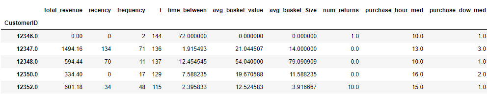
Now you data is in the format that each row is indexed by a unique CustomerID and the features are some sort of aggregations of the transactional data we had previously. Make sure to follow the get_features function and understand the aggregations that happened there. Now, our data is in the format that we can use for modelling.
DNN Model
Here, I’m going to use a Keras API to Tensorflow to build a simple DNN. Architecture here doesn’t really matter because the problem is simple and small enough. However, if you have more data, make sure to fine tune the model. Start small, and see if the performance increases as the complexity increases.
#DNN
def build_model():
    model = keras.Sequential([
    layers.Dense(256, activation='relu', input_shape=[len(X_train.columns), ]),
    layers.Dropout(0.3),
    layers.Dense(64, activation='relu'),
    layers.Dropout(0.3),
    layers.Dense(32, activation='relu'),
    layers.Dense(1)
    ])

    optimizer = tf.keras.optimizers.Adam(0.001)

    model.compile(loss='mse',
            optimizer=optimizer,
            metrics=['mae', 'mse'])

    return model

# The patience parameter is the amount of epochs to check for improvement
early_stop = keras.callbacks.EarlyStopping(monitor='val_mse', patience=50)

model = build_model()
#Should take 10 sec
early_history = model.fit(X_train, y_train,
                    epochs=1000, validation_split = 0.2, verbose=0,
                    callbacks=[early_stop, tfdocs.modeling.EpochDots()])
And that’s it! Now, you can predict revenue generated by a customer in the next 3 months given the features from the previous 160 days. But is this model any good? Let’s try to find out in the evaluation section.
Evaluation
There are two ways that I’m going to evaluate the model:
- This model can be evaluated as any other regression problem using metrics such as MSE/MAE or R2 scores
- DNN model can also be evaluated by comparing it to BG/NBD model results
def evaluate(actual, sales_prediction):
print(f"Total Sales Actual: {np.round(actual.sum())}")
print(f"Total Sales Predicted: {np.round(sales_prediction.sum())}")
print(f"Individual R2 score: {r2_score(actual, sales_prediction)} ")
print(f"Individual Mean Absolute Error: {mean_absolute_error(actual, sales_prediction)}")
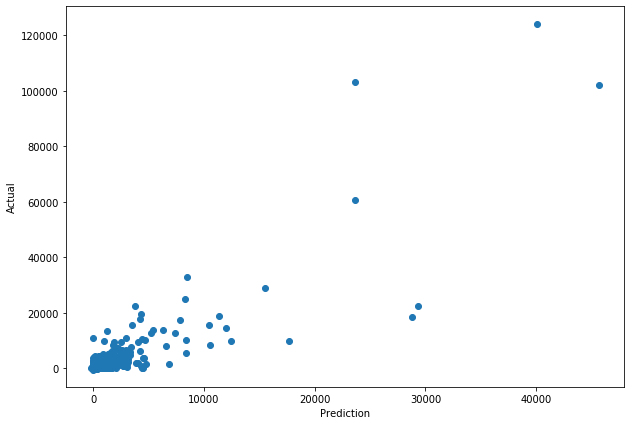
plt.scatter(sales_prediction, actual)
plt.xlabel('Prediction')
plt.ylabel('Actual')
plt.show()
#Predicting
dnn_preds = model.predict(X_test).ravel()
evaluate(y_test, dnn_preds)
From the evaluation print, we can see that the model underpredicts the total number of sales but this is likely due to the large outliers that the model can’t predict. You should get the R2 score between 0.5 and 0.7 which is good enough to conclude that our model makes meaningful predictions. MAE achieved here is quite large as well, but this again is due to the outliers. If you want, you can perform similar evaluation excluding outliers, and you’ll get much better results in terms of MSE or MAE. Here’s the scatter plot where we can see that the outliers and we can confirm that those with larger CLV are also generally predicted to have larger CLV.
Comparing DNN to BG/NBD
I’ll attempt to compare the performance of DNN and BG/NBD models by looking at:
- How well do they fit the non-outlier distribution
- How much revenue do the top customers according to CLV generate
I’ve covered BG/NBD modelling step-by-step in my previous blog, so here, I’ll just include the code. The notebook in my github repo goes a bit deeper into each step as well, so feel free to refer to it if you don’t understand what’s happening.
##PRE-PROCESSING
#Context data for the revenue (date & customerID)
id_lookup = data[['CustomerID', 'InvoiceNo', 'date']].drop_duplicates()
id_lookup.index = id_lookup['InvoiceNo']
id_lookup = id_lookup.drop('InvoiceNo', axis=1)
transactions_data = pd.DataFrame(data.groupby('InvoiceNo')['Revenue'].sum()).join(id_lookup)

#Spit into train - test
rfm_train_test = calibration_and_holdout_data(transactions_data, 'CustomerID', 'date',
                                        calibration_period_end='2011-09-10',
                                        monetary_value_col = 'Revenue')

#Selecting only customers with positive value in the calibration period (otherwise Gamma-Gamma model doesn't work)
rfm_train_test = rfm_train_test.loc[rfm_train_test['monetary_value_cal'] > 0, :]

##TRAINING
#Train the BG/NBD model
bgf = BetaGeoFitter(penalizer_coef=0.1)
bgf.fit(rfm_train_test['frequency_cal'], rfm_train_test['recency_cal'], rfm_train_test['T_cal'])

#Train Gamma-Gamma
print(rfm_train_test[['monetary_value_cal', 'frequency_cal']].corr())
ggf = GammaGammaFitter(penalizer_coef = 0)
ggf.fit(rfm_train_test['frequency_cal'],
        rfm_train_test['monetary_value_cal'])

##PREDICTION
#Predict the expected number of transactions in the next 89 days
predicted_bgf = bgf.predict(89,
                        rfm_train_test['frequency_cal'],
                        rfm_train_test['recency_cal'],
                        rfm_train_test['T_cal'])
trans_pred = predicted_bgf.fillna(0)

#Predict the average order value
monetary_pred = ggf.conditional_expected_average_profit(rfm_train_test['frequency_cal'],
                                        rfm_train_test['monetary_value_cal'])

#Putting it all together
sales_pred = trans_pred * monetary_pred
It should be noted that the datasets to train the models do differ a bit. E.g. some customer IDs had to be dropped because of their returns so the expected value was replaced by 0 in BG/NBD. Still, I’m not looking at the prediction on the user level but at the aggregate so this should not affect the evaluation. Also, seeing that the outliers affect the evaluation so much, I’ll exclude them to make it more understandable. First, let’s look at the distributions of predicted vs actual.
#First 98.5% of data
no_out = compare_df.loc[(compare_df['actual'] <= np.quantile(compare_df['actual'], 0.985)), :]
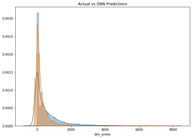
#Distribution of DNN
sns.distplot(no_out['actual'])
sns.distplot(no_out['dnn_preds'])
plt.title('Actual vs DNN Predictions')
plt.show()
#Distribution of BG/NBD + Gamma-Gamma
sns.distplot(no_out['actual'])
sns.distplot(no_out['stat_pred'])
plt.title('Actual vs BG/NBD Predictions')
plt.show()
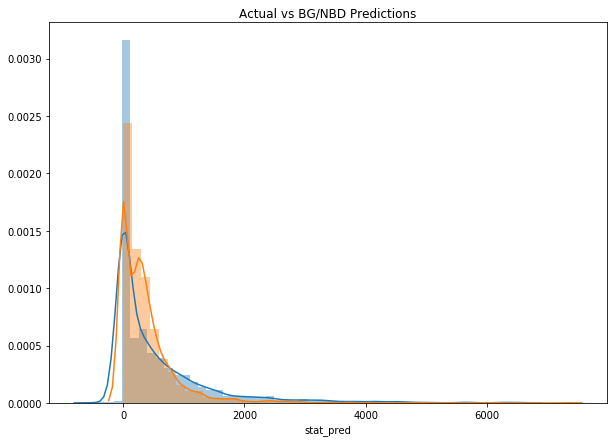
It looks like both models correctly model the revenue as heavily skewed with long tail. Nevertheless, DNN seems to better fit the data as it doesn’t have this second spike. Let’s now look at the revenue of top 20%.
top_n = int(np.round(compare_df.shape[0] * 0.2))
print(f'Selecting the first {top_n} users')

#Selecting IDs
dnn_ids = compare_df['dnn_preds'].sort_values(ascending=False).index[:top_n].values
stat_ids = compare_df['stat_pred'].sort_values(ascending=False).index[:top_n].values

#Filtering the data
eval_subset = data.loc[data.date >= '2011-09-10', :]

#Sums
dnn_rev = eval_subset.loc[eval_subset.CustomerID.isin(dnn_ids), 'Revenue'].sum()
stat_rev = eval_subset.loc[eval_subset.CustomerID.isin(stat_ids), 'Revenue'].sum()


print(f'Top 20% selected by DNN have generated {np.round(dnn_rev)}')
print(f'Top 20% selected by BG/NBD and Gamma Gamma have generated {np.round(stat_rev)}')
print(f'Thats {np.round(dnn_rev - stat_rev)} of marginal revenue')
The difference is only 6,134 (you’ll get different answer) which is quite insignificant. Hence, both methods are able to effectively pick the top 20% of most valuable customers which is not surprising, given that we’ve used only the transactions data in our DNN model. What about the first 10%? If you run the code cell above and replace 0.2 with 0.1, you’ll get your answer. For me, the DNN model customers have generated less revenue but also by only a small percentage (1.3%). Hence, the conclusion from this experiment and comparison is - Given only the transactions data, both DNN’s performance is similar to the BG/NBD + Gamma-Gamma approach.
Conclusion
In this blog, you saw how you can approach the CLV problem as ML regressions task. We’ve delved into feature engineering for such tasks, trained a 3 layer DNN, and evaluated it. The comparison to a simpler statistical approach have shown no particular advantage of using DNN for this particular dataset. In general, this conclusion is quite relevant for a lot of data science tasks: use the simplest technique that fits the task and achieves good results. But, if you have access to a lot more data and a lot more personal features, makes sure to experiment with the ML approach.
![]()