Who doesn’t have a good story about a time when the tracking broke down and conversions went to 0 for about a week before anyone noticed? In this case you lose a lot of precious data but it can be much worse. For example, let’s say your “Add to Cart” link is broken and the actual sales go down, or the discount code reduces the price to 0% and the sales sky-rocket for some reason. These technical issues have a real impact on business and can be quite costly. While an analyst will easily see where the problem has occured just by looking at the graph, he/she can’t possible monitor all the metrics available. Wouldn’t it be nice, if there was a way to automatically detect these abnormalities in your time-series data? Well, you’re in luck! In this 2 part blog series, I’ll walk you through 6 of these techniques, will show you how to implmenet them in Python, and will compare them on a few benchmark datasets.
Unsupervised Anomaly Detection
Anomaly detection can be defined as identification of data points which can be considered as outliers in a specific context. In time-series, most frequently these outliers are either sudden spikes or drops which are not consistent with the data properties (trend, seasonality). Outliers can also be shifts in trends or increases in variance. This problem can be approached in supervised (with labeled data) and unsuperised fashion (without labeled data). However, in the most real-life scenarios, access to the labeled data is scarce and the anomalous patterns may change. Due to these two reasons most of the businesses (that I know of) choose to implement the unsupervised models. In this blog, we’ll cover 3 unsupervised methods (in part 2 we’ll cover another 3), namely:
- Rolling Averages
- Auto-Regressive (AR) Models
- Seasonal Models
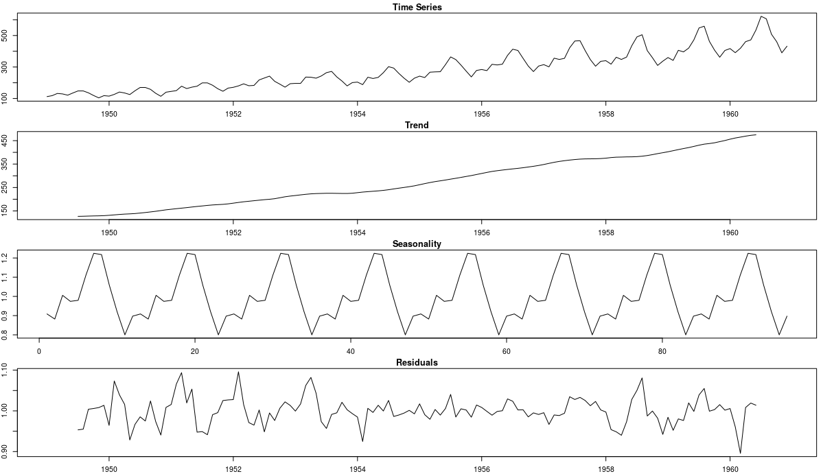
These algorithms are time-series specific and are based on time-series properties. Rolling Averages approach compares the rolling average at time t with the previous values of the average, and if the difference gets too large - the point gets flagged as outlier. The Auto-Regressive approach to anomaly detection is more sophisticated and builds an AR model to explain the time-series. Then it finds the residuals which are above a certain threshold and these become our outliers. Seasonal Model makes use of a classical econometrics technique called seasonal decomposition (see below). It separates trend and seasonality from the data which leaves us again with the residuals. Then we apply the same appraoch as with AR model and find the outliers.
Now that we have an overview of these techniques, let’s see how they perform on website traffic data.
Setup
You can download website traffic from this Kaggle competition. In addition, if you want to run the benchmarks yourself and see the performance, you can download the labeled dataset here. I’ll try to post all the code here but some bits might be missing. So, go to my github page if you want the entire notebook. I’m going to be using 3 main libraries for anomaly detection - ADTK(Part 1), scikit-learn (Part 2), and HDBSCAN(Part 2). You can pip install them with no isses. With the setup complete, we can read in the data and see how it looks like.
Data
#Read in the data
df = pd.read_csv('./data/wiki_ts.csv')
print(f'There is {df.shape[0]} websites, with visitis between {df.columns[1]} and {df.columns[-1]}')
#Filter out the time-series with NA values
no_nas = df.loc[(df.isna().sum(axis=1) == 0), :]
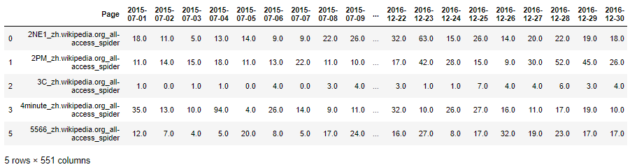
no_nas.head()
The first two lines should print There is 145063 websites, with visitis between 2015-07-01 and 2016-12-31. The data here is represented as dataframe with each row being the web traffic time-series for a particular website. After filtering out the time-series with NA values, here’s how the data should look like:
Because there’s so many websites, we’re only going to focus on 2 random websites in the further analysis. Let’s select these two websites and plot them.
#Select 2 random websites
wiki_sample = no_nas.sample(random_state=42).iloc[:, 1:]
x = pd.to_datetime(wiki_sample.columns.ravel())
y = wiki_sample.values.ravel()

wiki_sample = no_nas.sample(random_state=33333).iloc[:, 1:]
x2 = pd.to_datetime(wiki_sample.columns.ravel())
y2 = wiki_sample.values.ravel()

#Plot the website data
plt.title(f'Web Traffic for {no_nas.sample(random_state=42).iloc[:, 0].values[0]}')
sns.lineplot(x, y)
plt.show()

plt.title(f'Web Traffic for {no_nas.sample(random_state=33333).iloc[:, 0].values[0]}')
sns.lineplot(x2, y2)
plt.show()
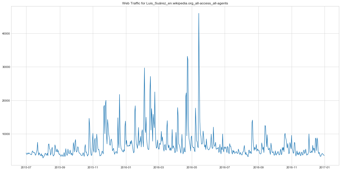 This timeseries representes the traffic on the Luis Suarez wikipage (he’s footabl player for Barcelona). It has quite a few spikes, which might be explained by the footbal season activity and his performance in the matches. For example, detecting these spikes might be useful in forecasting demand for his merchendise.
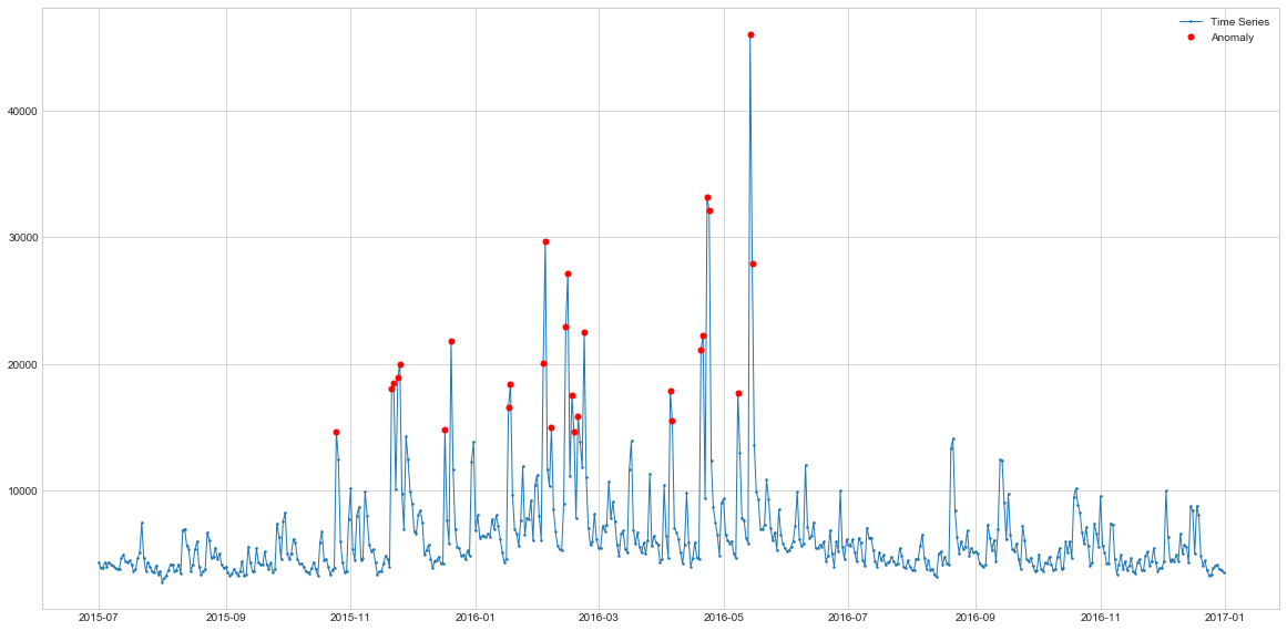
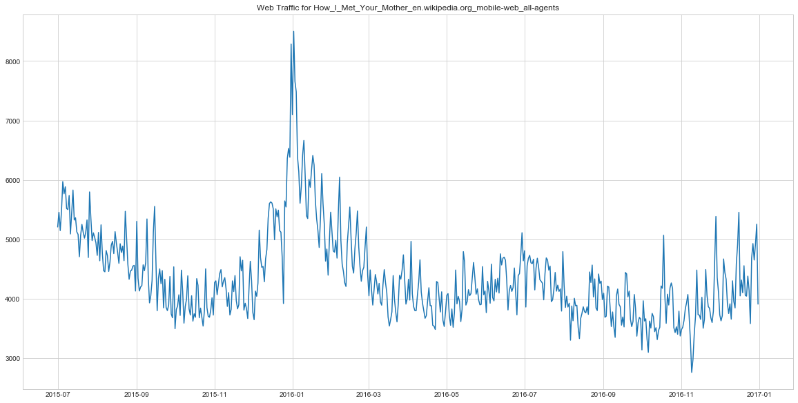 This time series is for a TV-show How I Met Your Mother. We can see that it has some sort of a seasonal pattern which might be connected to the broadcasting scheduel. Understanding the anomalies here might be useful in evaluating the success of different episode.
Let’s see which data points in these two series are considered abnormal by different algorithms.
Anomaly Detection with ADTK
adtk is a Python package that has quite a few nicely implemented algorithms for unsupervised anomaly detection in time-series data. In particular, we’re going to try their implementations of Rolling Averages, AR Model and Seasonal Model. These three methods are the first approaches to try when working with time-series. Rolling average (denoted as persistAD in adtk package) is the simplest of these approaches but it can work surprisingly well when the data is not very complicated. When the Rolling Average approach fails, Auto-Regressive and Seasonal approaches may performa better because most of the time-series are indeed generated by the auto-regressive processes, and some of them have a seasonal component.
Rolling Averages
persistAD has one main attribute to adjust - window. Window defines the length of the preceeding time window with which you’re going to compare the current value of your rolling average. Window of 1 will result in the detection of very short-term anomalies, whereas larger values (e.g. 30) will detect long-term outliers. In this case, I picked the number 7 as suitable because we have daily data and seasonality is likely to be weekly. In addition, parameter c can also be adjusted but it simply determines the bound of normal values, so the higher it is, the less outliers it will find. Here’s how you implement it in practice:
#Transforming data into Series with Timestamp index
s1 = pd.Series(data=y, index=x)
s2 = pd.Series(data=y2, index=x2)

#Initilise the detector
persist_ad = PersistAD(window=7, c=3, side='both')

#Detect anomalies
anomalies1 = persist_ad.fit_detect(s1)
anomalies2 = persist_ad.fit_detect(s2)

#Plot anomalies (with adtk plot method)
plot(s1, anomaly=anomalies1, ts_linewidth=1, ts_markersize=3, anomaly_color='red', figsize=(20,10), anomaly_tag="marker", anomaly_markersize=5)
plot(s2, anomaly=anomalies2, ts_linewidth=1, ts_markersize=3, anomaly_color='red', figsize=(20,10), anomaly_tag="marker", anomaly_markersize=5)
 Here I’m using 7 day rolling averages to find the outliers. We can see that the highlighted points are indeed spikes in the time-series and could be considered as outliers. Hence, the simplest approach already does a pretty good job at finding the anomalies. However, it also flags some of the data points that follow the spikes as outliers as well, which might be incorrect. Maybe adjusting the window parameter would help to deal with this issues. Let’s see how it performs with more seasonal data of the website 2.
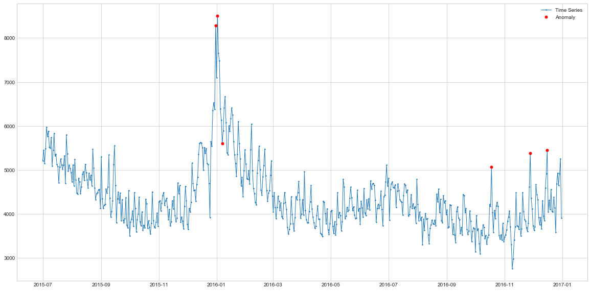 Here, the model also picks up the main outlier spikes (christmas and new year) and it also highlights some of the spikes closer to the end of time-series. You will need some business context to understand whether these are indeed outliers or they were mislabeled. But overall, the Moving Average approach does a decent job at this dataset as well. Let’s see how does the Seasonal Model perform on these two datasets.
Seasonal Model
The only parameter that seasonalAD needs is the freq. This paramter determines the frequency of the dataset which helps it to find the appropriate seasonality. It can be inferred automatically but your data must have no missing periods.
#Initialise the detector
seasonal_ad = SeasonalAD(c=3.0, side="both")

#Detect anomalies
anomalies_season1 = seasonal_ad.fit_detect(s1)
anomalies_season2 = seasonal_ad.fit_detect(s2)

#Plot anomalies
plot(s1, anomaly=anomalies_season1, ts_linewidth=1, ts_markersize=3, anomaly_color='red', figsize=(20,10), anomaly_tag="marker", anomaly_markersize=5)
plot(s2, anomaly=anomalies_season2, ts_linewidth=1, ts_markersize=3, anomaly_color='red', figsize=(20,10), anomaly_tag="marker", anomaly_markersize=5)
 Comparing to Rolling Averages approach, Seasonal model is a lot more consistent in the outliers it identifies. These are the spikes which do not match seasonal pattern. That’s why we can see some of the spikes not highilghted - these are seasonal spikes and not outliers. In this sense, the model highlights less points, but these points are more likely to be outliers.
 Here again, the key outliers are highlighted meaning that the spike during the Christmas period of 2015 is abnormal. But the seasonal model doesn’t highlight the December 2016 spikes, meaning that these spikes are in-line with seasonal expectation of a model. If we look closely at the time series, we can see that indeed during the December period wee can expect larger number of visits. Hence, the Seasonal model again is more likely to be correct than simple Moving Averages.
Auto-Regressive Model
To use the AR model, we first need to determine the number of lags to use. For this, we can use ACF plots.
acf = plot_acf(s1, lags = 60)
acf = plot_acf(s2, lags = 60)
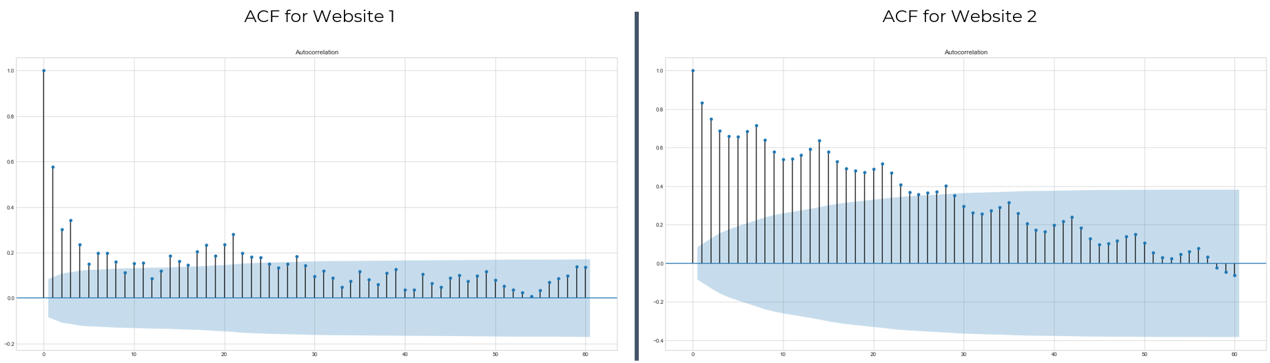
Looks like including 30 time steps will be enough to capture the time-dependence of this time-series. Hence, the n_steps parameter in AutoregressionAD is set to 30. The detection procedure is very similar to the previous methods.
#Initilaise detector
autoregression_ad = AutoregressionAD(n_steps=30, step_size=1, c=3.0)

#Detect anomalies
anomalies_ar1 = autoregression_ad.fit_detect(s1.resample('D').sum())
anomalies_ar2 = autoregression_ad.fit_detect(s2.resample('D').sum())

#Plot anomalies
plot(s1, anomaly=anomalies_ar1, ts_linewidth=1, ts_markersize=3, anomaly_color='red', figsize=(20,10), anomaly_tag="marker", anomaly_markersize=5)
plot(s2, anomaly=anomalies_ar2, ts_linewidth=1, ts_markersize=3, anomaly_color='red', figsize=(20,10), anomaly_tag="marker", anomaly_markersize=5)
 The AR model is able to capture spikes and performs quite similarly to the Rolling-Average approach. So it also finds some of the points right after the spikes as abnormal which looks incorrect. It also misses some of the spikes at the end of the series.
 On this dataset, AR finds two areas of anomaly, similar to the Rolling Average. However, while the Rollign Average has identified multiple points closer to the end of the series, AR only finds one spike.
Conclusion
In this blog you saw how you can easily implement 3 different algorithms for anomaly detection in time-series data. Because the dataset is not labelled we cannot conclude which method performs the best on these series, but we can see the differences between the detected data points. Ultimately, it all depends on how does your website traffic data look like and what particular outliers you want to detect. This checklist should somewhat help you in determining the methodology to use:
- Is there seasonality in your data? - If yes, try Seasonal Model
- Is your data auto-correlated? - If yes, try Auto-Regressive Model
- Is your data noisy? - If yes, try Rolling Averages
- Are you looking for local or more global outliers? - If local - use Rolling Averages with small window. If global - use larger window.
Also, keep in mind that these are only 3 out of 13 anomaly detection methods of adtk library. Make sure to check out their documentation with example to see any other methods might be more suitable to your data.
The next part is going to cover more ML based detectors such as Local Outlier Factor, GLOSH, and Isolation Forest, so stay tuned.