In part 1 of this blog series I’ve talked about more classical approaches to anomaly detection. They utilise some of the time-series’ properties (moving averages, auto-regression, seasonality) and they are quite efficient and accurate. However, there might be cases when we need to add some additional context variables (e.g. type of products, weather) that are relevant to the task or when these algorithms are unable to detect some outliers. In these cases, it’s good to have additional algorithms in your toolkit that use somewhat different approaches in detecting the anomalies. Here, I’m going to cover 3 new algorithms:
- Local Outlier Factor (LOF)
- Global Local Outlier Score in Hierarchies (GLOSH)
- Isolation Forest
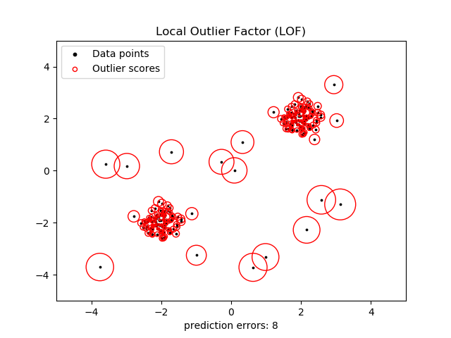
The two first models are based on the concepts of distance and density. LOF algorithm (Breunig et al., 2000) gives each point a density score which is determined by its proximity to other data points. Proximity is usually measured by Euclidean distance but it can be other metric as well. Clusters with very high density are considered to be normal, whereas points which belong to the regions with lowest density are considered to be outliers. GLOSH (Campello et al., 2015) is further improvement of this approach and it based on hierarchical estimates. These two approaches work in practice because they can detect local outliers. This means that they will flag not only the most obvious spikes and drops but they will also detect outliers in specific contexts (e.g. holidays) that can look abnormal.
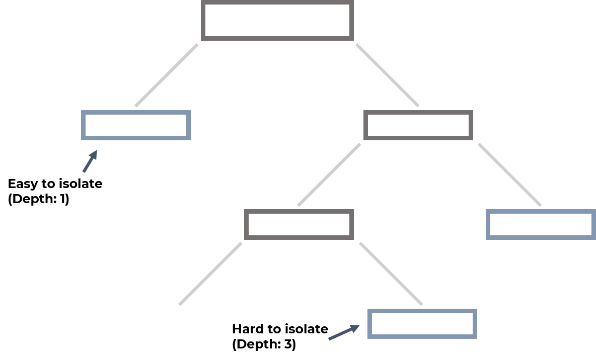
Finally, Isolation Forest (Liu et al., 2008) is a tree-based method that builds a number of decision trees and parses through the data chossing the best splits (based on entropy or information gain). It then measures how deep a tree has to be for a data point to be isolated, averages this depth score across the trees, and find the outliers. Outliers are those with the smallest depth score because they were among the easiest to be isolated (e.g. in the first or second splits).
Setup
Setup is similar to the last part, so you can simply continue working the in the same notebook. If you haven’t followed Part 1, you can follow the setup instructions there and come back here after installing the dependencies, downloading the data, and reading it in. I’m going to use the sklearn implementation of LOF and their implementation of Isolation Forest. For GLOSH algorithm we can use the HDBSCAN implementation.
Models
In this section I’m going to show you how you can fit these models on web-traffic data and how the results can be visualised. Afterwards, these models are going to be benchmarked on a variety of labelled time-series datasets. We’ll start with the density-based models.
LOF
Thankfully, sklearn’s API is intuitive and well documented, so fitting the model is quite easy. The only parameter that you might want to provide is the contamination rate which helps the algorithm to understand how many outliers you expect to find. This will determin the boundaries that the LOF builds. Here, we’re going to use the default auto but if you know approximately the proportion of outliers, feel free to provide it.
#Imports for context (not needed if you're following the notebook, as they've been imported previously)
from sklearn.neighbors import LocalOutlierFactor
from adtk.visualization import plot

clf = LocalOutlierFactor(contamination='auto')
lof_outliers1 = clf.fit_predict(np.array(s1).reshape(-1,1))
lof_outliers1 = pd.Series([x == -1 for x in lof_outliers1], index=s1.index)
plot(s1, anomaly=lof_outliers1, ts_linewidth=1, ts_markersize=3, anomaly_color='red', figsize=(20,10), anomaly_tag="marker", anomaly_markersize=5)
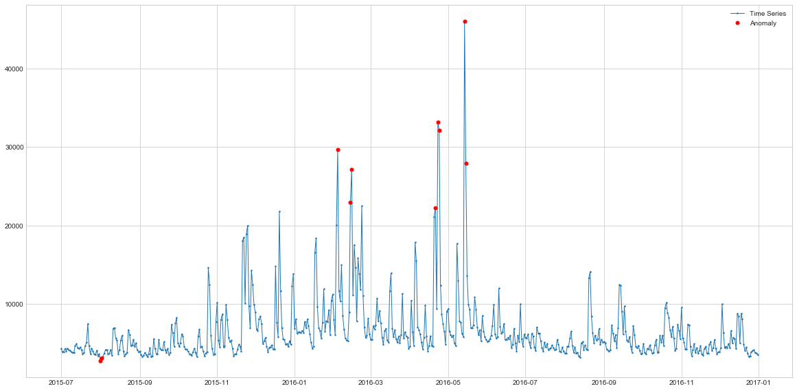
With default parameters, the LOF algorithm doesn’t tag some of the spikes but it detects two datapoints at the start of time-series which were previously never considered as outliers. This might be the local context property of the algorithm, as these points at the start seem to indeed be lower than expected. The spikes, on the other hand, seem to be in-line with local expectations of that time-series period Let’s see how it does at the seasonal data.
lof_outliers2 = clf.fit_predict(np.array(s2).reshape(-1,1))
lof_outliers2 = pd.Series([x == -1 for x in lof_outliers2], index=s2.index)
plot(s2, anomaly=lof_outliers2, ts_linewidth=1, ts_markersize=3, anomaly_color='red', figsize=(20,10), anomaly_tag="marker", anomaly_markersize=5)
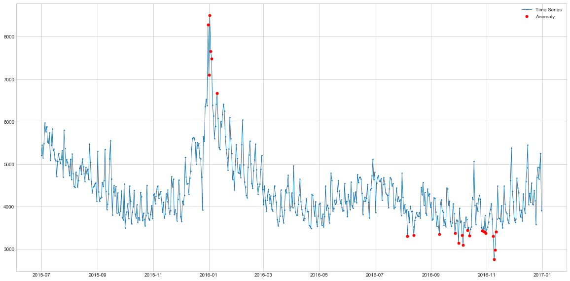 Here the performance is again in-line with what we saw previously. It finds the main outlier peak and it also detects the lower points at the end of the series. Because these points are indeed lower than anything we have seen in the series, they might be considered as anomalies or, at least, they should be detected. Overall, this algorithm has provided a new perspective on our time-series data simply because it uses another logic under the hood. This just further illustrates how important it is to know your data and your expected outliers.
GLOSH
Because HDBSCAN is density-based algorithm, they’ve provided an easy way of calculating the outlier scores according to GLOSH algorithm. Let’s see how we can get these scores and what to do next with them
import hdbscan

#Fit the clustering model
clusterer = hdbscan.HDBSCAN(min_cluster_size=15).fit(np.array(s1).reshape(-1,1))

#Series 2
clusterer2 = hdbscan.HDBSCAN(min_cluster_size=15).fit(np.array(s2).reshape(-1,1))

#Plot the outlier scores
sns.distplot(clusterer.outlier_scores_[np.isfinite(clusterer.outlier_scores_)], rug=True)
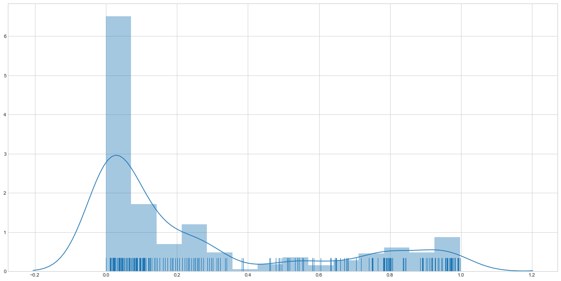
This is the distribution of outlier scores for the first web traffic dataset. As you can see, the majority of data points have very low score which means that they are highly unlikely to be outliers. Our task now is to choose the thresholds for both websites which will determine above which outlier score do we consider a point to be an anomaly? Here, I’m going to use just 90th percentile cut-off but make sure to experiment and take into account your business goals before making this decision.
#Define the threshold
threshold = pd.Series(clusterer.outlier_scores_).quantile(0.9)
#Find points above the threshold
outliers = np.where(clusterer.outlier_scores_ > threshold)[0]
outliers = s1[outliers]
#Plot them
outliers_series = pd.Series(s1.index.isin(outliers.index), index=s1.index)
plot(s1, anomaly=outliers_series, ts_linewidth=1, ts_markersize=3, anomaly_color='red', figsize=(20,10), anomaly_tag="marker", anomaly_markersize=5)
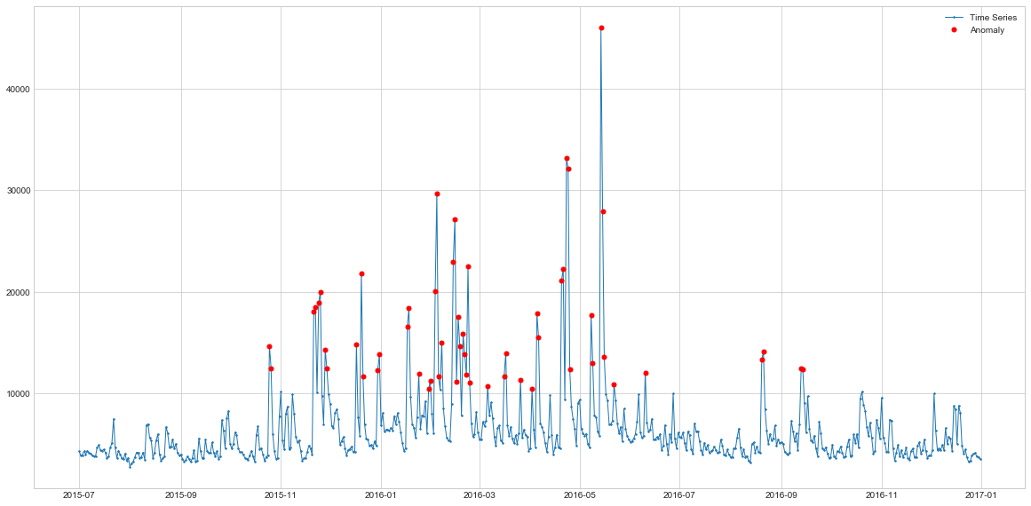
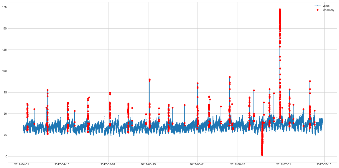
The HDBSCAN does a pretty good job at detecting the spikes and it’s also more consistent as it detects mostly the spikes and not the falls after the spikes. Actually, the performance looks quite similar to the seasonal model with addition of a few spikes which is quite interesting. In comparison to LOF, its outliers are more global which makes sense due to the nature of this algorithm.
#Same process as above
threshold2 = pd.Series(clusterer2.outlier_scores_).quantile(0.90)
outliers2 = np.where(clusterer2.outlier_scores_ > threshold2)[0]
outliers2 = s2[outliers2]
outliers_series2 = pd.Series(s2.index.isin(outliers2.index), index=s2.index)
plot(s2, anomaly=outliers_series2, ts_linewidth=1, ts_markersize=3, anomaly_color='red', figsize=(20,10), anomaly_tag="marker", anomaly_markersize=5)
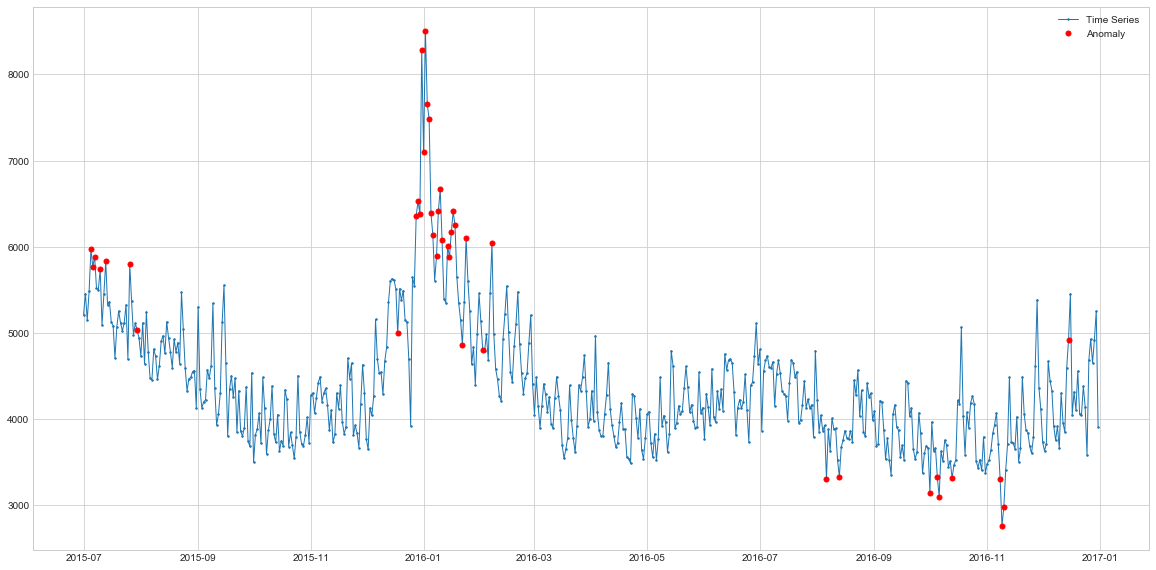 Interstingly, on this dataset, in addition to spikes HDBSCAN also detects the sudden drops which the classical detection approaches have missed. On the other hand, it also seems to mislabel some points at the beginning of the series, so it might be an indiciation that we need to increase the quantile from 90% to e.g. 95% or 98%. Here again, business context is key in determining these thresholds as the output has to be useful to the end users and decision makers.
Isolation Forest
This models also has quite an intuitive implementation in sklearn and the only parameter is to specify is again the contamination rate.
from sklearn.ensemble import IsolationForest

clf = IsolationForest(contamination='auto', behaviour="new")
if_outliers1 = clf.fit_predict(np.array(s1).reshape(-1,1))
if_outliers1 = pd.Series([x == -1 for x in if_outliers1], index=s1.index)
plot(s1, anomaly=if_outliers1, ts_linewidth=1, ts_markersize=3, anomaly_color='red', figsize=(20,10), anomaly_tag="marker", anomaly_markersize=5)
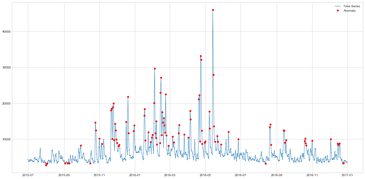 Interestingly, Isolation Forest is able to detect both spikes and drops, and it flags way more datapoints as outliers than previous algorithms. Let’s see its behaviour on another web traffic data.
if_outliers2 = clf.fit_predict(np.array(s2).reshape(-1,1))
if_outliers2 = pd.Series([x == -1 for x in if_outliers2], index=s2.index)
plot(s2, anomaly=if_outliers2, ts_linewidth=1, ts_markersize=3, anomaly_color='red', figsize=(20,10), anomaly_tag="marker", anomaly_markersize=5)
Here again, it flags a lot of points as outliers with its default parameters. Hence, we might want to lower the contamination rate for it to be more conservative.
Evaluation on Labelled Dataset
So far, we’ve seen 6 algorithms (including the previous part) and each of them detects slightly different type of outliers. While there’s clearly no one-size-fits-all approach to this problem, it’d be good to see their performance on a variety of datasets and have some sort of a benchmark study. Exactly for this reason, I’m going to use a labeled dataset from this competition to calculate the F1 scores of different anomaly detection algorithms for a variety of time-series. Let’s read in the data and see how one of the series looks like.
train = pd.read_csv('./data/phase2_train.csv')

#select a series
kpi = 'c69a50cf-ee03-3bd7-831e-407d36c7ee91'
kpi_train = train.loc[train['KPI ID'] == kpi, :]
#From timestamp to date
kpi_train.timestamp = kpi_train.timestamp.apply(lambda x: datetime.fromtimestamp(x))
kpi_train.index = kpi_train.timestamp

#Proportion of anomalies
print(kpi_train['label'].value_counts(normalize=True))
#only 0.6% of points are anomalies

plot(kpi_train.value, anomaly=kpi_train['label'], ts_linewidth=1, ts_markersize=3, anomaly_color='red', figsize=(20,10), anomaly_tag="marker", anomaly_markersize=5)
So here the data is quite seasonal most of the annomalies are sudden spikes or falls after them. In theory, a simple moving average filter should be able to deal with most of them, but our goal is to find the algorithm which works the best across multiple time-series. Hence, let’s now use the models discussed on this and 28 other time-series.
#Defining a new class using the the functions from before
class SeriesAnomalyDetector:
    def rolling_avg(self, data, window):
        persist_ad = PersistAD(window=window, c=3, side='both') #Compares 2 hours means
        persist_anomalies = persist_ad.fit_detect(data)
        return persist_anomalies.fillna(0)

    def ar(self, data, n_steps, step_size):
        autoregression_ad = AutoregressionAD(n_steps=n_steps, step_size=step_size, c=3.0)
        ar_anomalies = autoregression_ad.fit_detect(data)
        return ar_anomalies.fillna(0)

    def seasonal(self, data):
        seasonal_ad = SeasonalAD(c=3.0, side="both")
        season_anomalies = seasonal_ad.fit_detect(data)
        season_anomalies = season_anomalies[data.index]
        return season_anomalies.fillna(0)

    def hdbscan(self, data, q):
        clusterer = hdbscan.HDBSCAN(min_cluster_size=15).fit(np.array(data).reshape(-1,1))
        threshold = pd.Series(clusterer.outlier_scores_).quantile(q)
        hdbscan_outliers = np.where(clusterer.outlier_scores_ > threshold)[0]
        hdbscan_outliers = data[hdbscan_outliers]
        hdbscan_anomalies = pd.Series(data.index.isin(hdbscan_outliers.index), index=data.index)
        return hdbscan_anomalies.fillna(0)

    def lof(self, data, c):
        clf = LocalOutlierFactor(contamination=c)
        lof_outliers = clf.fit_predict(np.array(data).reshape(-1,1))
        lof_anomalies = pd.Series([x == -1 for x in lof_outliers], index=data.index)
        return lof_anomalies.fillna(0)

    def isolation_f(self, data, c):
        clf = IsolationForest(contamination=c, behaviour="new")
        if_outliers = clf.fit_predict(np.array(data).reshape(-1,1))
        if_anomalies = pd.Series([x == -1 for x in if_outliers], index=data.index)
        return if_anomalies.fillna(0)
As you can see from the code, I’m cheating a little bit by providing the actual contamination % . Then, to get actually unbiased results, I’d have to test these algorithms on the test set with the same contamination rates for LOF and Isolation Forest. I’m not going to do this here, but feel free to try it at your own (there is testing dataset at the link as well). The actual detection code looks as follows:
from tqdm import tqdm
#Saving the proportion for later testing
contamination_dict = {}
performance = {}

for kpi in tqdm(train['KPI ID'].unique()):
    #Data Selection
    filt_df = train.loc[train['KPI ID'] == kpi, :]
    filt_df.timestamp = filt_df.timestamp.apply(lambda x: datetime.fromtimestamp(x))
    filt_df.index = filt_df.timestamp
    #Time cleaning (sometimes required)
    filt_df = filt_df.sort_index()
    filt_df = filt_df.loc[~filt_df.index.duplicated(keep='first')]
    c = filt_df['label'].value_counts(normalize=True)[1]
    q = 1-c
    data = filt_df.value.resample(pd.infer_freq(filt_df.index[:5])).sum()

    #Anomaly detection
    detector = SeriesAnomalyDetector()
    ra = detector.rolling_avg(data, 60)
    ar = detector.ar(data, 60, 1)
    try:
        seasonal = detector.seasonal(data)
    except:
        seasonal = pd.Series(index=data.index).fillna(False)
    hdb = detector.hdbscan(data, q)
    lof = detector.lof(data, c)
    isolation_f = detector.isolation_f(data, c)
    f1_scores = []
    anomalies = [ra, ar, seasonal, hdb, lof, isolation_f]
    methods = ['Rolling Average', 'Auto-Regressive', 'Seasonal Model', 'HDBSCAN', 'LOF', 'Isolation Forest']
    for i, a in enumerate(anomalies):
        f1_scores.append(f1_score(filt_df.label.values, a[filt_df.label.index]))
        print(f'{methods[i]} F1 score: {f1_score(filt_df.label.values, a[filt_df.label.index])}')

    #Storing parameters and results
    contamination_dict[kpi] = c
    performance[kpi] = f1_scores

#Average Performance
performance_df = pd.DataFrame(performance).transpose()
performance_df.columns = methods
performance_df.describe()
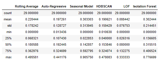
Now this table is interesting because if we look at the averages, Seasonal Model and Isolation Forest perform the best. However, Seasonal model’s standard deviation is quite large and so if we look at the median values, Isolation forest is a clear winner, followed by Auto Regressibve and Rolling averages models. This indicates that when the seasonal model is applicable, it has the best performance but, unfortunately, not all the cases have seasonal patterns so it can fail miserably sometimes. To do some visual evaluation, let’s the the time-series where models have performed the best.
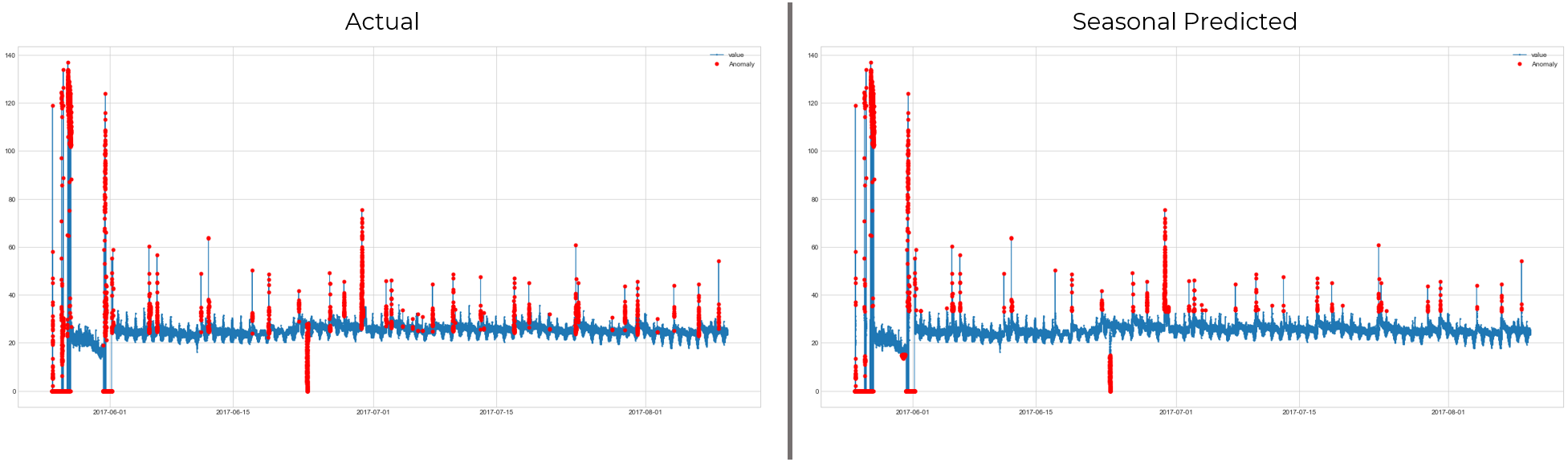 Here the data clearly has seasonal patterns, so the seasonal model is the best choice here. Setting simple thresholds or using rolling averages wouldn’t work here, so detecting seasonality in these kinds of data is crucial. Now, let’s see where seasonal model won’t help us in finding the anomalies and isolation forest is a better choice.
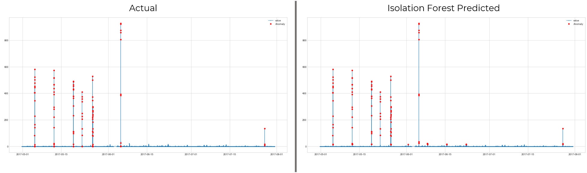
Here isolation forest does quite well and it’s not surprising. This case has no seasonality and the outliers are clearly visible.There’s no context to understand, so 1 feature isolation forest is ineed the best choice. Let’s see where it fails to perform well.
Conclusion
In this blog you’ve seen 3 new unsupervised anomaly detection algorithms. Two of them are based on the idea of distance and density while the Isolation Forest is a completely novel algorithm relying on the number of splits. As you saw in the example, each algorithm detects somewhat different type of outliers, so make sure to understand your data and experiment before choosing the algorithm. From the comparison on labelled dataset, we saw that Isolation Forest and Seasonal Models have better performance than other algorithms but again, they have quite large standard deviations and work for some datasets while failing on other ones. Hence, when you are working with other datasets, you can start with these two models, get the benchmark, and begin your exploration.
In the next and final part of the unsupervised anomaly detection blogs I’m going to explore how you can detect the anomalies using Autoencoders. Stay tuned on my github and linkedin profile to not miss it.