Propensity modelling is a process of assigning propbabilities to commit a certain action (e.g. to buy, to churn, etc.) to each individual in your customer base using statistical models. Hence, we can think of it as a classification problem which can be solved using a multitude of ML models. When could these models be used? Propensity scores allow marketing managers to tailor their communications and offers on the individual level. Knowing if a customer is going to buy in the next month can help us formulate the type of communications that he/she is going to receive. For example, if we know that this high propensity customer enjoys a particular category of products, we can send tailored recommendations to this customer’s email which is going to imporve the customer’s experience with our brand. On the other hand, if we know that a customer is likely to churn, we can offer a special discount to encourage the customer to stay.
Bottom line: propensity models form a crucial pillar in marketing analytics and are extremely valuable to the business. Let’s see now how can we make the process of propensity modelling in Python as easy as possible.
Setup
If you want to follow along this blog you download the notebooks from my repo. The data that for this tutorial can be downloaded from Kaggle, but feel free to use your own data as well. Two main packages used for data preparation were developed by Feature Labs, the open-source hand of Alteryx. These packages are ComposeML and Featuretools and you can install them via regular pip install. The package used for modelling is called PyCaret - open-source low-code library for rapid prototyping and development of ML models. I highly recommend that you make a clean environment before installing PyCaret because it has a lot of dependencies which might conflict with your current versions.
Objective
What kind of propensity are we going to predict? Well, if you look at the EDA section in the notebook, you can see that customers make pruchases quite freuqently, so propnesity to buy in the next month or week would not be very useful for this business. Hence, instead of predicting if a person is going to make pruchase, we are going to predict if the number of transactions is going to be larger than average. We’re also going to do it on the weekly level as it gives more detailed insights and can still be actionable for marketing managers. The only thing that we need to specify is the threhsold above which we’lll classify the customer as super customer for the next week. Let’s take a look at the distribution of weekly number of purchases.
#How many items do people purchase weekly?
transactions = pd.read_csv('./data/customer_transaction_data.csv', parse_dates=[0])

#group by id and date
transformed_data = pd.DataFrame(transactions.groupby(['customer_id', 'date'])['quantity', 'selling_price'].sum()).reset_index()

#How many items do people purchase weekly?
weekly_purchases = transformed_data.groupby(['customer_id', pd.Grouper(key='date', freq='W-MON')])['quantity'].sum().reset_index().sort_values('date')
weekly_purchases['quantity'].describe()
75th percentile make more than 49 weekly purchases, so this is going to be our threshold. Hence, the main objective of this tutorial is to predict if a customer is going to make more than 49 purchases in the following week
Data Preparation
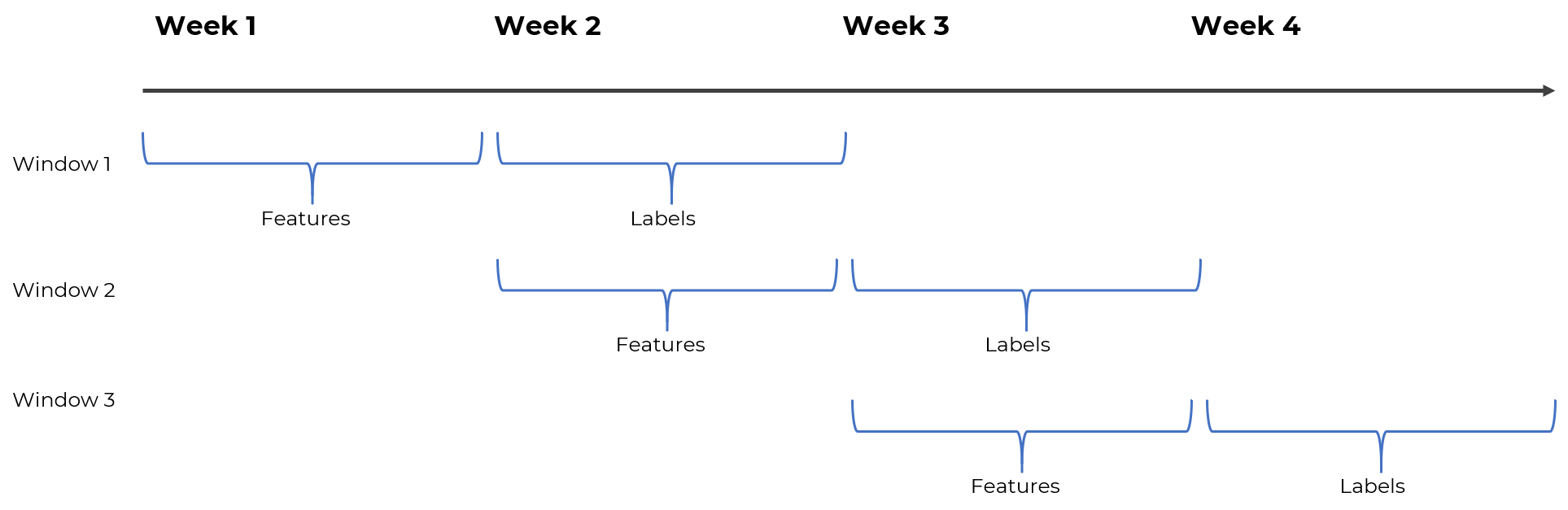
This section is split into two parts: label engineering and feature engineering. The data preparation process is quite complicated because we’re dealing with moving windows of data, and hence need to be careful to include only the data from the relevant dates. For example, this is how windowing would work if we were trying to forecast the next week based on the previous week’s actions.
Label Engineering
First, let’s create a function that is going to implement the logic of being a “super-customer”. As stated previosuly, we’re going to label people as positive examples if their weekly number of transactions is above 49.
def is_super(df):
    total = df['quantity'].sum()
    if total > 49:
        return 1
    else:
        return 0
Next, we’re going to use composeml class called LabelMaker. It will take care of windowing for us, so the only thing that we need to do is to provide all the right parameters. If you are unsure about any of the parameters, read the documentation or drop a comment in this article.
import composeml as cp

#Creating LabelMaker instance
label_maker = cp.LabelMaker(
    target_entity="customer_id", #for whom to create labels?
    time_index="date",
    labeling_function=is_super, #scoring function above
    window_size="W" #weekly window
)

#Crating labels
lt = label_maker.search(
    transactions.sort_values('date'),
    minimum_data='2012-07-02', #date where the first label will be created
    num_examples_per_instance=-1, #its flexible
    verbose=True, #will show a progress bar
    drop_empty=False #don't drop the weeks with no purchase
)

lt.head()
This should take about a minute, and at the end you should see this table printed out.
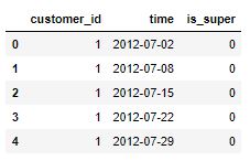
As you can see, each label corresponds to a particular customer ID and date. Hence, multiple labels are created for each customer according to the windowing approach. This was quite easy, right? Let’s see now how can we create corresponding features for these labels.
Feature Engineering
Here I’m going to use featuretools to automatically create complicated features on the various sliding windows. The first step in this process is to set-up a schema with entities that you have (just like in database development). If you’re using the data from Kaggle, this is how the actual schema looks like:
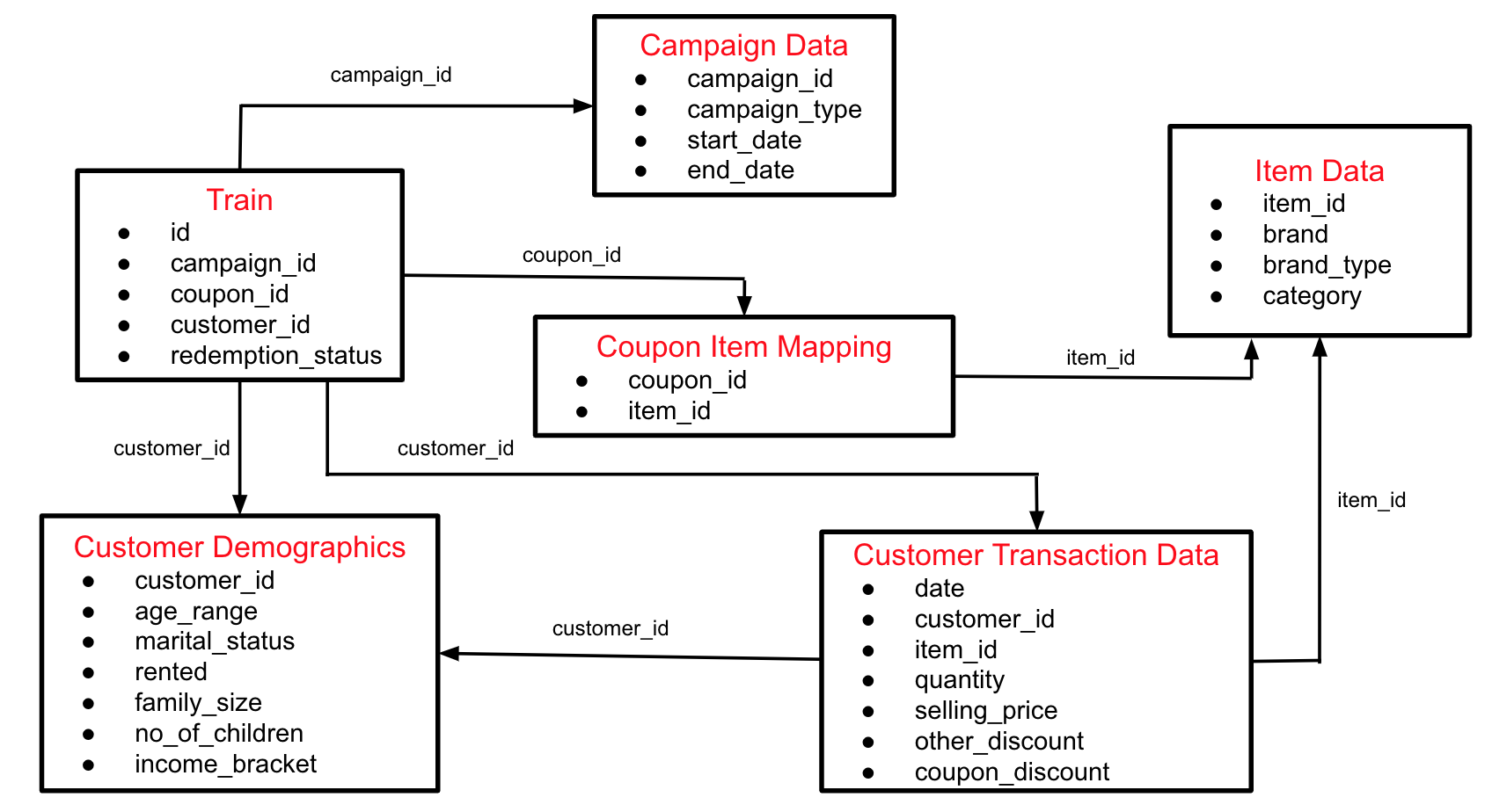
For now, we’ll use only 3 of these tables - transactions, customers, and items. You can see that customers and items are connected to the transactions table via the key columns. Featuretools needs this information to connect these tables and create meaningful features using Deep Feature Syntehsis.
#Creating entity set
es = ft.EntitySet(id="customer_data")

#Each dataset should have a unique ID column, so for transactions we need to create it and remove any duplicates. Here I'm going to use the combination of date, customer id, #and item id.
#Concatenate the fields to create ID
transactions['transaction_id'] = transactions.date.astype(str) + '_' + transactions.customer_id.astype(str) + '_' + transactions.item_id.astype(str)
#Remove duplicates
transactions_cleaned = transactions.drop_duplicates(subset='transaction_id')
#Select only relevant features
transactions_cleaned = transactions_cleaned[['transaction_id', 'date', 'customer_id', 'item_id', 'quantity', 'selling_price',
       'other_discount', 'coupon_discount']]

#Adding Transactions Table
es = es.entity_from_dataframe(entity_id="transactions", #just a name for table
                              dataframe=transactions_cleaned, #actual dataframe
                              index="transaction_id", #column with unique ID
                              time_index="date", #date columns
                              variable_types={"item_id": ft.variable_types.Categorical}) #make sure to specify categorical

#Adding Items Table
 es = es.entity_from_dataframe(entity_id="items",
                             dataframe=items,
                             index="item_id",
                             variable_types={"brand": ft.variable_types.Categorical}) #make sure to specify categorical

#Adding Customers Table
es = es.entity_from_dataframe(entity_id='customers',
                             dataframe=customers,
                             index='customer_id',
                             variable_types={"rented": ft.variable_types.Categorical,
                                            "no_of_children": ft.variable_types.Categorical,
                                            "income_bracket": ft.variable_types.Categorical})
Now we have all the tables in our schema but they are not connected yet. To add the connections, we have to specify which columns act as common key between the tables (just like in SQL joins).
#Connecting Items to Transactions
rel1 = ft.Relationship(es["items"]["item_id"], #common key in Items
                                      es["transactions"]["item_id"]) #common key in Transactions
es = es.add_relationship(rel1)

#Connecting Customers to Transactions
rel2 = ft.Relationship(es["customers"]["customer_id"], #common key in Customers
                                      es["transactions"]["customer_id"]) #common key in Transactions
es = es.add_relationship(rel2)

#print the schema
print(es)
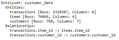
Check in the print out that all the needed tables were added and the relationships are correctly specified. With schema in place, we can finally move to feature engineering. I’m going to use the very basic features of this amazing package, so make sure to read the documentation and experiment with the parameters. They can play a huge role in the further results.
Since I’m making weekly predictions, my features will also be on the weekly level. In particular, the features are going to be created for the windows of 7, 14, 21, 28, 35, 42, 49, and 56 days. This is probably an overkill so make sure to experiment with the time-windows to find the ones which fit your dataset the best. I’m going to make a for loop to iterate the windows and use the dfs class to generate features.
day_windows = [7, 14, 21, 28, 35, 42, 49, 56] #all the window frames
feature_dfs = [] #to populate with features
feature_encodings = []

for w in day_windows:
    feature_matrix, features = ft.dfs(target_entity="customers",
                                  cutoff_time=lt, #the labels created earlier
                                  training_window=ft.Timedelta(f"{str(w)} days"), #Window populated in the for loop
                                  ignore_variables = {'customers': [c for c in customers.columns[1:]]}, #ignore demographic variables
                                  max_features = 20, #number of features to generate per window
                                  entityset=es, #schema created before
                                  verbose=True
                                 )

    feature_matrix.columns = [f'D{str(w)}_' + c for c in feature_matrix.columns] #renaming columns to merge
    feature_matrix = feature_matrix[[c for c in feature_matrix.columns if 'is_super' not in c]] #excluding the label column to not get duplicated
    feature_dfs.append(encoded) #populating the list above
    feature_encodings.append(features) #saving for later use


#Joining all features
all_features = pd.concat(feature_dfs, axis=1)

#Adding label column
all_features['is_super'] = lt['is_super'].values

#Saving the data for training
all_features.to_csv('./outputs/generated_data.csv')

print(all_features.head())
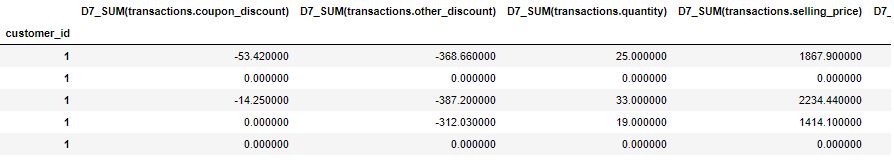
Overall, your dataset is going to have 161 columns - 160 features (8 windows * 20 features) and 1 label. So, each label from the LabelMaker output gets a bunch of corresponding features which is a perfect setup for classical Machine Learning classifciation task.
Classifciation with PyCaret
Modelling in PyCaret in general is very experiment focused (as any DS project should be in the beginning). So you need to get used to the experimenting framework that it provides, luckily it’s quite intuitive and easy to use. The Modelling process will consist out of the following steps:
- Setup the experiment parameters which include
- Data cleaning
- Data transformation
- Dimensionality reduction
- and a lot more…(see the documentation for all the options)
- Compare the available models and pick the best ones
- Tune the models
- Try Ensembles and Stacking
- Evaluate
- Save the model
- Run another experiment until you are satisfied with the preformance
Experiment Setup
When you setup an experiment in PyCaret, you have an opportunity to specify how you want your data to be pre-processed and transformed. There’s a wide range of options but I’ll use only some of them. In particular I will:
- Normalise and transform the input features - to make sure that data satisfies the requirements of all the models
- Remove multicollinear features - to reduce the number of columns
- Apply Principal Component Analysis - to reduce the dimensionality
- Apply SMOTE - to fix the imbalance in labels
#Read in the previously created features
data = pd.read_csv('./output/generated_data.csv')
#Read in the customer dataset
customers = pd.read_csv('./data/customer_demographics.csv')

#Add the customer data to previously created features
data_with_demo = data2.merge(customers, on='customer_id', how='left')

#Specify the experiment parameters
clf = setup(data_with_demo, target = 'is_super', session_id=123, log_experiment=True, experiment_name='with_demo_pca',
             train_size=0.7,
             normalize = True,
             transformation = True,
             ignore_low_variance = True,
             remove_multicollinearity = True,
             multicollinearity_threshold = 0.95,
             categorical_features = ['marital_status', 'rented', 'family_size', 'no_of_children', 'age_range', 'income_bracket'], #numeric to categorical
             pca=True, pca_components=0.95,
             fix_imbalance=True)
Running this cell will start the process where you’ll have to, first, confirm that the column types were inferred correctly and, second, will need to choose the % of your dataset to be used in modelling. Sometimes it makes sense to use all the datase and sometimes the subset will be fine to evaluate the performance of different models. It all depends on the quality of signal in your dataset and the complexity of your problem, so use the evaluation plot provided in the process to make your decision. Note: the model will be fitted on all the data when you finalise it, so the subset will only be used during the model comparison and evaluation. After the setup is complete, you’ll see the following table which allows you to see all the parameters that you’ve specified.
![]()
Modelling
The best to start modelling in PyCaret is by comparing all the models in its arsenal to establish a baseline and the best type of models suited for your data. One line of code and you have an estimate of your model’s performance. Amazing, right? You can select how many best-performing models do you want to save with n_select parameter, and what evaliation metric to use to measure the performance with the parameter sort. Here, I’m going to save 5 best models and use AUC score to sort them.
top_models = compare_models(sort='AUC', n_select=5, fold=10)
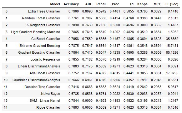
The table above is going to be automatically generated. As you can see, tree-based models are much better at dealing with this problem than parametric models with Extra Trees Classifier achieving the best AUC score of 0.81. These scores are based on 10-fold cross-validation. Can we do better than 0.81 AUC? Let’s try with hyperparameter tuning.
Model Tuning
Hyperparameter tuning is also a one-line command in PyCaret. In the background it uses a Random Grid Search with pre-defined search space which is not the optimal strategy to use, but it is very easy and efficient. Important parameters to consider:
- n_iter - default is 10, but if you have time set it to 50-100
- custom_grid - if you know what you are doing, provide your own grid
- optimize - metric to optimise, by default Accuracy in classification. Set it to AUC for binary or F1 for multi-class
- choose_better - will replace a model only if found a better model. By default is False, but set it to True.
#Tuneing all 5 best models
tuned_best = [tune_model(m, n_iter=20, optimize='AUC', choose_better=True) for m in top_models]
With the models tuned, we can try squeezing extra points of performance using ensembles or stacking. We can do ensebmle modelling using the blend_models method in PyCaret. It simply takes the outputs of all the input models and creates a soft (with probability) or hard (0 or 1) voting classifier. If majority of models vote yes, the example is considered as positive, and vice versa. Note: CatBoost is incompatible with Voting Classifier
blended = blend_models(estimator_list = tuned_best[:4], method = 'soft') #doesn't take catboost yet
As we can see, we’ve achieved an increse in AUC from 0.8096 to 0.8175 just by running 2 lines of code. It’s not a huge increase, but can be important in the real-life scenario.
Evaluation
Evaluation in PyCaret is done on the hold-out dataset, so the model has never seen this data before. The most common way to evaluate the binary classifciation problem is by using ROC curve and confusion matrix. Luckily, both of these graphs (and a lot more) are implemented in PyCaret so drawing them is quite easy. By calling plot_model(blended) you will get the following ROC curve:
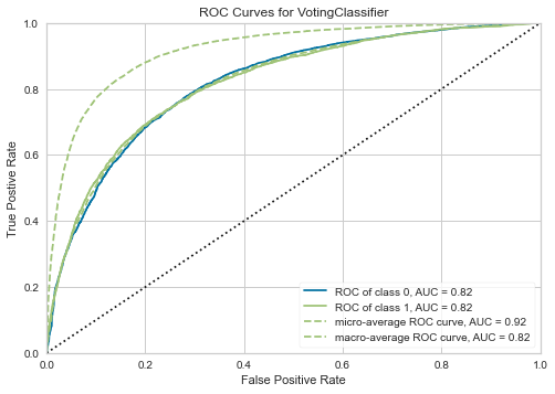
The holdout AUC is 0.82 so it has generalised well from the training set. From the graph we can pick the acceptable level of True Positive and see the corresponding rate of False Positives. You can also plot the confusion matrix by running plot_model(blended, plot='confusion_matrix') line of code. By default, the probability threshold is 0.5 but I want to adjust it, so I will make my own predictions on the hold-out dataset and will plot the confusion matrix. I want to correctly classify about 60% of super customers which corresponds to ~0.25 threshold.
#Hold out predictions
holdout_predict = predict_model(blended, probability_threshold = 0.25) #set new threshold

labels = [0,1]
cm = confusion_matrix(holdout_predict['is_super'], holdout_predict['Label'], labels, normalize='true')
ax= plt.subplot()
sns.heatmap(cm, annot=True, fmt='.2', ax = ax); #annot=True to annotate cells

# labels, title and ticks
ax.set_xlabel('Predicted labels');ax.set_ylabel('True labels');
ax.set_title('Confusion Matrix');
ax.xaxis.set_ticklabels(['Regular', 'Super']); ax.yaxis.set_ticklabels(['Regular', 'Super']);
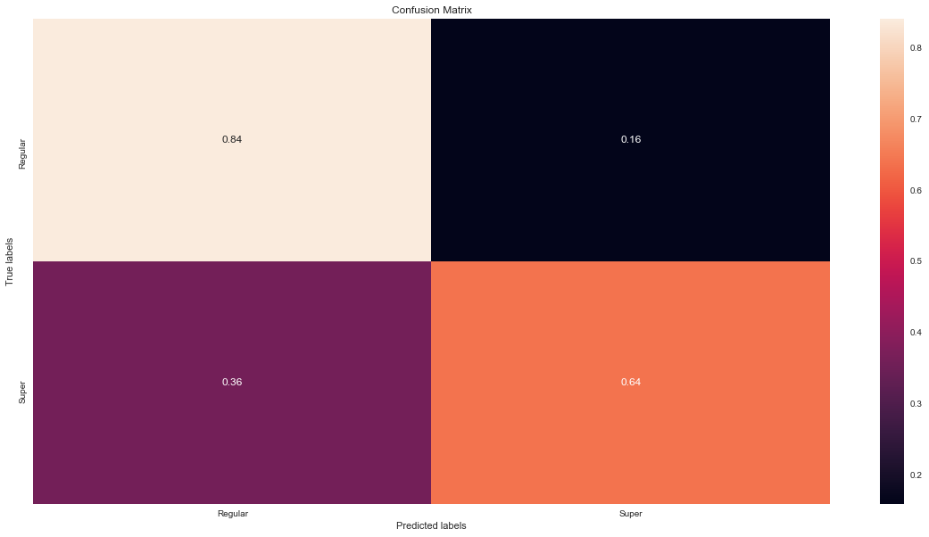
As you can see, our model is now able to classify correctly 64% of super-customers but it also misclassifies 16% of regular customers. This is by far not the best model that we could have created, but given that it was built using only a few lines of code and automatically engineered features, it is a great result and a solid first step in the data science project.
Conclusion
In this article we’ve set out to build a model that can predict if a customer is going to make more than 49 purchases in the following week. While building this model you saw how you can use composeml to generate time-windowed labels, and featuretools to automatically generate corresponding features. Next we’ve compared a large variety of models and picked the top 5. After tuning and ensembling, we’ve ended up with a decent model in a record low number of lines of code. You can keep experimenting with feature engineering by adding seeded features, increasing the depth of features, or using more complicated primitives. You can also keep improving the model by changing the pre-processing parameters, trying stacking, or using custom hyperparameter grids. Let me know how far you managed to imporve the results!
Feel free to write comments, share this blog, or write to me directly with your thoughts. Also, let me know if you want me to cover any other marketing related data science topic.